Chapter 14 Step-by-step tutorial :
Re-creating the SIR module
This second tutorial demonstrates that the EvoLudo simulation toolkit also provides a powerful framework for modelling classical epidemiological processes. More specifically, the SIR module implements the standard model for describing the spread of a disease in a population. It divides the population into three compartments: the susceptible individuals, , that are prone to infection, the infected individuals, , that carry the disease and may transmit it to others, and the recovered individuals, , that have recovered from the disease and developed resistance against it.
The classical approach to analyze the dynamics in the model is to use ordinary differential equations (ODE) (XXX). The dynamical equations describe the rate of change of the frequencies in the three compartments , , and , respectively. The simplest way to derive the dynamics is to consider basic reactions between members of the three compartments:
| (14.1a) | ||||
| (14.1b) | ||||
| (14.1c) | ||||
| (14.1d) | ||||
The first reaction describes the infection of susceptible individuals by infected ones, which happens at rate and moves individuals from the susceptible to the infected compartment. The second and third reactions describe the recovery of infected individuals. The difference is that at rate individuals develop immunity and join the resistant compartment, while at rate they simply return to the susceptible compartment. The last reaction describes the loss of immunity of recovered individuals at rate , which places them again into the susceptible compartment.
Based on the mass-action principle, the reactions in Eq. (14.1) can be immediately translated to a system of ODE’s for the dynamics of the densities in the three compartments , , and :
| (14.2a) | ||||
| (14.2b) | ||||
| (14.2c) | ||||
| . | . | Note: The number of types on both sides of the reactions in Eq. (14.1) are equal. This implies that the overall population density remains constant and is reflected in the fact that in Eq. (14.2), or, equivalently . | . |
Because the overall population density is conserved, the dynamics of the three compartments can be reduced to a two-dimensional system of ODE’s. More specifically, the dynamics of any one compartment can be expressed in terms of the other two compartments. For example, the dynamics of the infected individuals can be expressed as:
| (14.3) |
This means there are only two independent dynamical variables and the third is a dependent variable because it can be expressed in terms of the other two. However, we are free to choose which variable is the dependent one. Moreover, without loss of generality, we can normalize the population density to one and express the dynamics in terms of their frequencies. This also means that the dynamics actually unfolds on the simplex spanned by the three compartments, but more on this later.
As a warm-up exercise, let us solve the model analytically first, and calculate the equilibria and basic reproduction number, , which determines whether the disease can spread in the population or not. Later we can use these results to check the numerical output of EvoLudo.
-
Exercise 14.1:
Calculate the frequencies of the three compartments at all equilibria of Eq. (14.2).
Solution There are two equilibria, a disease-free equilibrium, , with , and , or with any mixture of and , if resistance does not wear off, . The second, endemic equilibrium, , is given by -
Exercise 14.2:
Calculate , which denotes the basic reproduction number of the disease and is defined as the expected number of secondary infections produced by a single infected individual. The disease can spread in the population if .
Hint corresponds to the growth rate of the disease in the early stages of the epidemic and is given by the per-capita growth rate of the infected compartment, in the limit . Solution -
Exercise 14.3:
What fraction of the population of susceptible individuals needs to be vaccinated to prevent the disease from gaining a foothold in the population as a function of the rate of infection, ?
Hint must hold. Vaccinated people fall into the resistant compartment. Solution or the fraction needs to be vaccinated. The more infectious the disease, the higher the fraction of vaccinated individuals must be to achieve herd immunity.
The equilibrium is called an endemic equilibrium, provided that , because the disease persists in the population, that is, it becomes endemic.
14.1 Create the module
As in the case of the TBT module, the SIR module implements a set of interfaces that define the underlying process and advertise the ways to visualize the dynamics, see Fig. 14.1.
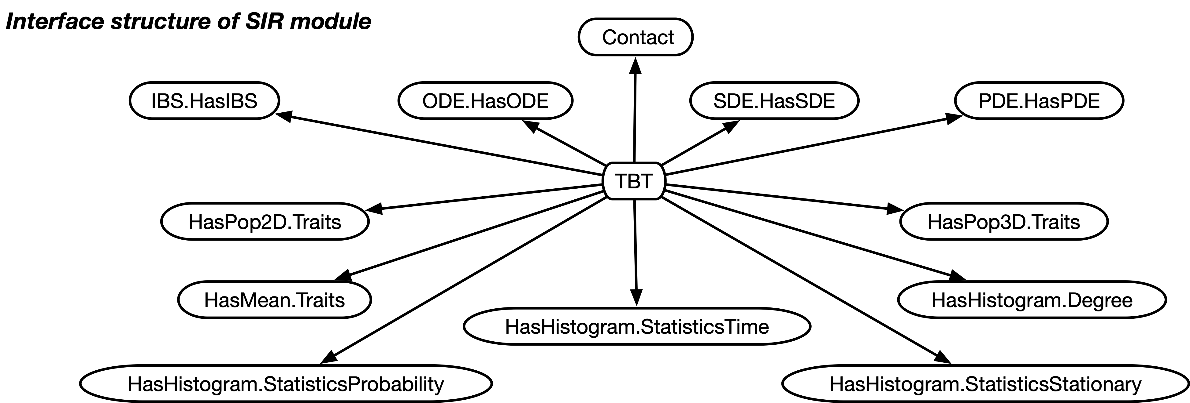
The capabilities of the SIR module are advertised and specified through the following interfaces:
- Discrete
-
for discrete individual traits (or types, or compartments),
- HasIBS
-
for individual based simulations, IBS,
- HasDE.ODE
-
for deterministic dynamics based on ordinary differential equations, ODE,
- HasDE.SDE
-
for stochastic dynamics based on the Euler-Maruyama method (ODE with a stochastic noise term),
- HasDE.PDE
-
for deterministic dynamics in spatial settings modelled by partial differential equations, PDE, based on the Euler method combined with a reaction-diffusion term.
Moreover, the SIR module implements the following interfaces to request a set of GUI views to graphically visualize various aspects of the dynamics:
- HasPop2D.Traits
-
display the types of all individuals in a 2D plot (IBS and PDE only),
- HasPop3D.Traits
-
display the types of all individuals in a 3D plot (IBS and PDE only),
- HasMean.Traits
-
plot the mean frequency of each type over time,
- HasHistogram.Degree
-
plot the degree distribution of the population structure (IBS and PDE only),
- HasHistogram.StatisticsStationary
-
plot the histogram for the sojourn time for the different type counts in the stationary distribution.
This tutorial guides you through the process of creating a new module from scratch but will eventually be identical to the existing SIR module. Since module names (as well as java class names) must be unique, we have to choose a name other than SIR. Let’s use SIRE – appending an E for EvoLudo.
| . | . | Note: On a case-sensitive file system you can get away with using, for example, the class and file name SiR instead of SIRE because java is case-sensitive. However, this is not recommended because it jeopardizes the portability of the code. | . |
The initial steps to create a new module are essentially the same as in the previous tutorial, chapter 13: Step-by-step tutorial : Re-creating the TBT module. In order to get started, create a new java file org.evoludo.simulator.modules.SIRE in the EvoLudoCore maven module. In VS Code right-click on the modules folder in EvoLudoCore/src/main/java/org/evoludo/simulator and select New Java File ¿ Class…. Enter the name of the new file as SIRE. The new file should look like this: The initial steps to create a new module are essentially the same as in the previous tutorial, chapter 13: Step-by-step tutorial : Re-creating the TBT module. In order to get started, create a new java file org.evoludo.simulator.modules.SIRE in the EvoLudoCore maven module. In VS Code right-click on the modules folder in EvoLudoCore/src/main/java/org/evoludo/simulator and select New Java File ¿ Class…. Enter the name of the new file as SIRE. The new file should look like this:
The following code snippets contain little to no comments because the SIR class serves as a reference file. Besides, the motivation and purpose of each code snippet is explained in detail in the accompanying text.
The new SIRE class must again extend the Discrete class because we are dealing with a discrete set of traits or types, say , , and . This is done by changing the class definition from SIRE to SIRE extends Discrete. The Discrete class provides a number of useful methods and fields to handle discrete traits. The Discrete class is located in the same package as the SIRE class, so no import statement is needed.
However, extending Discrete triggers two errors in VS Code because (i) the Discrete class does not provide a default constructor and (ii) SIRE does not implement the abstract method getTitle() of the Discrete class. Both errors are easily addressed in VS Code by hovering over the error location and selecting Quick fix…, followed by Add constructor SIRE(EvoLudo) as well as Add unimplemented methods.
| . | . | Note: The Discrete class has no default constructor and therefore subclasses must provide their own constructor using one of the constructors of the super class. All single species modules use the constructor Discrete(EvoLudo engine). | . |
Now the content of the file looks as follows:
In the constructor, there is nothing else we need to do, so simply delete the TODO comment.
| . | . | Note: If you follow the steps in this tutorial the line numbers in the code snippets should always match the line numbers in your file. | . |
The method getTitle() returns a short title of the module:
This information will be displayed in the list of available modules on the EvoLudo help screen. Before we can verify this, we need to make EvoLudo aware of the new module.
14.1.1 Adding the module to EvoLudo
In order to run the new module in EvoLudo, we first need to add it to the list of available modules (see also section 13.1.1: Adding the module to EvoLudo). This is done in the EvoLudo class: open org.evoludo.simulator.EvoLudo in the maven module EvoLudoCore, located in the parent directory of our SIRE class. The EvoLudo(boolean loadModules) constructor at the end of the file includes several addModule(...) calls to add all available modules. Add the following line to the list of modules:
together with the necessary import statement at the top:
Now that EvoLudo is aware of the new SIRE module, it can be compiled, launched and debugged in exactly the same manner as described in section 13.2: Running (and debugging) the module: simply exchange any occurrences of TxT with SIRE.
Last but not least, edit the file EvoLudoGWT/src/main/webapp/TestEvoLudo.html and look for the string <div class="evoludo-simulation" >. Change the data-clo attribute to "--module SIRE". This ensures that the SIRE module is loaded whenever the browser window is reloaded. Reload the page to recompiles EvoLudo. You should see a message similar to:
| . | . | Note: If you don’t see the message above you may need to apply the same edit to the EvoLudoGWT/target/EvoLudoGWT-1.0-SNAPSHOT/TestEvoLudo.html file. This is the file that the Jetty server sends to the browser. Alternatively, you can stop the Jetty server and run ’mvn clean install’ in the top level EvoLudo directory followed by ’mvn gwt:devmode’ to launch Jetty again. This recompiles all modules and copies the new TestEvoLudo.html file to the EvoLudoGWT/target/EvoLudoGWT-1.0-SNAPSHOT directory. | . |
The error that no model was found is expected, simply because we have not yet implemented a model. More importantly, the message ’Module loaded: Disease dynamics in EvoLudo’ indicates that the module has been successfully loaded. Thus, we can now start implementing the module.
14.2 Implementing the module
In essence, the model describes a contact process (durrett:XXX) with multiple types. In contrast to the tutorial, payoffs do not matter, and no game theoretical interactions take place between individuals. Instead, infected individuals may pass the infection to susceptible ones – should they come into contact. The other types can spontaneously convert to another type: infected ones recover, and recovered ones may lose resistance and become susceptible again. Since interactions with other types do not involve payoffs, SIRE does not implement the interface Payoffs and no further methods need to be implemented.
Let us start with some housekeeping. For convenience and to keep the code more readable, we define three constants for the indices of the different types:
Next, when loading a new module, the method load() is called and provides an opportunity to initialize the module. Most importantly, we must specify the number of types (or traits) by setting the field nTraits. Optionally, we may also set the names and colours of each trait. All this is done by overriding the method load():
The Color class requires another import statement at the top:
| . | . | Important: Don’t forget to call super.load() to allow parental classes to complete their own initializations. | . |
Since no memory was allocated in load(), no cleaning up is necessary when unloading the module and hence no need to override unload().
14.3 Adding ODE model:
ordinary differential equations
The classical model in the form of an ODE has already been derived in the introduction, see Eq. (14.2). So, let’s start with the implementation of the ODE model. As before, capabilities of an EvoLudo module are advertised by implementing the appropriate interfaces. In order to advertise the ODE model, we need to implement the HasDE.ODE interface:
together with the accompanying import statement:
The interface HasDE.ODE requires implementing one additional method, which is easily accomplished in VS Code by hovering over the error location and selecting Quick fix…, followed by Add unimplemented methods:
In modules where the overall population density remains constant and hence the dynamics can be expressed in terms of frequencies, the method getDependent() returns the index of the dependent trait. In principle, this can be any one of the three traits , , or . However, because the investigations will always focus on the infected or susceptible compartments, or , let’s choose as the dependent trait.
| . | . | Note: The model still makes sense without the compartment. For example, by setting and , the model reduces to the simpler model, where individuals are unable to develop immunity against the disease. | . |
In case the compartment is not relevant for the model, that is, if the trait is disabled, or no recruitment into the compartment happens, , the dependent trait should be , keeping the focus on the infected trait :
| . | . | Note: The method getDependent() could also return -1 to indicate that there is no dependent trait. The numerical integration would still work but runs an increased risk that the state ends up outside the simplex due to numerical errors. Declaring a dependent trait allows numerical adjustments to guarantee that the state remains inside . | . |
In order to implement the dynamical equations, Eq. (14.2), we need to define four additional fields that determine the transition rates between the different compartments, and assign them meaningful default values:
The exact values are not important but with those above, the infection becomes endemic and the disease persists in the population for most initial configurations.
What are the equilibrium frequencies of the three compartments? You can either solve Eq. (14.2) analytically by setting the left-hand side to zero and solve for the equilibria – or you can use EvoLudo to find the equilibria numerically. However, a few more steps are necessary before our module can accomplish this goal.
First and foremost we need to implement Eq. (14.2). This is done by defining a new inner class, say ODE, which extends the class org.evoludo.simulator.models.ODE.
| . | . | Note: In java it is possible to have several classes with the same name provided they are part of different packages and hence stored in different directories. In our case org.evoludo.simulator.models.ODE and the inner class org.evoludo.simulator.modules.SIRE.ODE we are about to create. When referring to ODE the one in the current file or specified in the imports list at the top is used. If another class of the same name needs to be referenced, the fully qualified name is required, e.g. org.evoludo.simulator.models.ODE. | . |
More precisely, the class org.evoludo.simulator.models.ODE implements a simple numerical integrator based on Euler’s method. However, we can do significantly better by extending the RungeKutta class, which uses the more sophisticated fifth-order Cash-Karp Runge-Kutta method with variable step size (Press et al., 2007).
Plus the corresponding import statement for the RungeKutta class:
As before, we can take advantage of VS Code’s Quick fix… feature to create a stub for the constructor:
Since nothing else needs to be done in the constructor, the TODO comment has already been deleted in the code snippet above.
Implementing the method getDerivatives(...)
Now we are ready to address the core issue and implement Eq. (14.2) by overriding the method getDerivatives(double t, double[] state, double[] unused, double[] change), which calculates the rate of change in each trait. The method takes four arguments to calculate the rates of change:
- t:
-
the time , only used in non-homogenous ODE’s (see section 14.9: Extension I: Adding seasonal variation for an example),
- state:
-
the array that represents the state of the population as specified by the respective densities/frequencies.
- unused:
-
an unused double array, which may be null (in modules that implement the interface Payoffs the array holds the fitness for each trait).
- change:
-
the array to return the rates of change .
Referring to Eq. (14.2), the rates of change are calculated as follows:
| . | . | Note: The advantage of using an inner class is to maintain direct access to all fields and methods of the outer class. In our case the parameters , , , and . | . |
The above code does not take advantage of the fact that the state is always normalized, , which implies that the sum of the rates of change must be zero. In order to improve accuracy and reduce numerical errors, we can
-
(i)
either calculate the rate of change of the dependent trait as the negative of the sum of the rates of change of the other two traits, or
-
(ii)
shift the rates of change to ensure they sum up to zero.
The first option singles out the dependent trait and treats it differently from the other two traits. The second option is more symmetric and hence preferable and can be implemented as follows:
A few comments on the details of the above code snippet are in order:
-
(i)
The variable psi is a helper variable to reduce access to entries in the array state.
-
(ii)
The rates are calculated separately in order to easily have a running sum of the rates of changes in the local variable totDelta, without having to access the entries in the array change.
-
(iii)
The variable accuracy denotes the desired numerical accuracy of the computation and can be set using the --accuracy <value> command line option. If the deviation from zero exceeds the desired accuracy, the rates of change are shifted by the average deviation, totDelta/nActive, where nActive denotes the number of active traits.
-
(iv)
The field active is a boolean array that indicates which traits are active. Traits can be deactivated using the --disable <index> command line option.
For more information on command line options, including --accuracy and --disable, see section 11.2: Parameters.
The final remaining task is to tell EvoLudo to use the newly minted custom class SIRE.ODE to run the ODE model. When loading the model, the EvoLudo engine calls the method createModel(Type type) in the Module class, where type refers to the requested type of model. By default, this method returns an instance of the class RungeKutta. To use our custom class instead, we simply need to override the createModel(Type type) in the SIRE module and return an instance of the inner class SIRE.ODE. In case the model already exists (and is of the right type), simply return the current model. Since no other models are currently supported, we return null for all other types:
At this point we now have a fully functional ODE model that can be used to simulate the dynamics of the model. In order to demonstrate this, consider the following exercise:
-
Exercise 14.4:
Determine the equilibrium frequencies of the three compartments , , and in the model with our default values for the transition rates.
Hint Simply click Start and observe the changes to the state of the population as summarized by the frequencies of the three types in the status line at the bottom of the EvoLudo GUI. After a few moments EvoLudo stops because the numerical integration has converged. Solution The equilibrium frequencies are , , and . -
Exercise 14.5:
Does the result depend on the initial conditions?
Hint Try different initial configurations using --init <s>,<i>,<r> in the EvoLudo settings. . . Note: If the arguments <s>,<i>,<r> do not add up to one, EvoLudo normalizes them. . Solution As long as there are at least some infected individuals initially, the disease will persist in the population and the equilibrium frequencies are independent of the initial conditions.
Note that the EvoLudo GUI includes a status line at the bottom that summarizes the current state of the population and displays the frequencies of individuals in the three compartments. Admittedly, this is a fairly underwhelming experience. Fortunately, EvoLudo provides a number of ways to visualize the dynamics of the model in more detail.
14.4 Adding GUI views
By default, the only view available in EvoLudo is the Console (see section 11.1.2: Views), which reports milestone events in the life cycle of a module (see section 12.10.1: Milestone listeners) as well as warnings and errors. Adding more detailed views is often as simple as implementing a particular interface.
14.4.1 Mean traits
In ODE models, the state of the population is fully determined by the frequencies of individuals in each compartment. This information is already displayed in the status line. However, it is much more informative to visualize the dynamics as a function of time. To request the view with the mean trait frequencies, all we need to do is implement the HasMean.Traits interface:
and the corresponding import statement at the top:
Give it a try by reloading the EvoLudo page in your browser to recompile the SIRE and display the Traits – Mean view.
14.4.2 Simplex
An alternate and often even more informative way to visualize the dynamics of the model is plotting the trajectory in the simplex spanned by the three compartments. Again, this is simply achieved by implementing another interface, HasS3:
and another import statement at the top:
Again, reload the page and switch to the Traits – Simplex view. A double click anywhere in the interior of the simplex conveniently sets the initial condition (provided the model is not running).
-
Exercise 14.6:
Verify that the equilibrium you found in Exercise 14.4 is located at , and demonstrate that is indeed a global attractor by generating trajectories from various initial conditions in the simplex .
14.5 Adding SDE model:
stochastic differential equations
With the successful implementation of the ODE model, adding a stochastic version of the model is rather straight forward. First we need to implement the HasDE.SDE interface to advertise to EvoLudo that the SIRE module also provides a model based on stochastic differential equations:
Just as for the ODE model, we now need to provide our own implementation of the SDE model. The part that is specific to the SIRE module are the rates of change that correspond to Eq. (14.2). Thus, let’s use the ODE model as a template and simply duplicate the inner class SIRE.ODE. Of course VS Code now complains about a duplicate nested type (SIRE.ODE). Simply replace all occurrences of ODE by SDE in the duplicated section to obtain:
Next, we need to return an instance of the inner class SIRE.SDE in the method createModel(Type type) by simply adding another if-condition:
Compile the module by reloading the EvoLudo page in your browser and verify that a new model is now available by clicking on Settings and Help. Now change to the SDE model by changing the EvoLudo settings to --model SDE and run the model. What are your observations?
Oops, quite clearly, the results are identical to the ODE model… What happened? Well, on closer inspection this is not surprising because we simply copied the ODE model!
| . | . | Important: Currently, our SDE model extends the RungeKutta class, which implements an ODE solver. Instead, we must extend the org.evoludo.simulator.models.SDE class, which adds demographic noise to mimic the dynamical process in finite populations. | . |
To fix this, we need to change the inner class SDE from extending RungeKutta to extend org.evoludo.simulator.models.SDE:
| . | . | Note: No additional import is needed because we provide the fully qualified class name, org.evoludo.simulator.models.SDE. This is necessary to prevent name clashes with our inner class of the same name, SIRE.SDE. | . |
Compile the SIRE module again and run the SDE model. Now you will see the expected noisy dynamics. The fixed point remains an attractor, but the trajectory fluctuates around it.
-
Exercise 14.7:
The demographic noise in the SDE model depends on the population size, which is by default. What happens if you increase the population size to , or even ?
. . Note: The population size is limited by the range of int variables in Java. The primitive type int has a maximum of or about . .
Hint Use the --popsize <N> setting to change the population size. Solution The noise scales with and hence gets smaller for larger . -
Exercise 14.8:
Does the population size affect the execution speed of the model?
Solution No. This is one of the key advantages of using SDE models over individual based simulations, IBS. -
Exercise 14.9:
How do the trajectories compare to the ODE results?
Solution Even for the trajectories are essentially indistinguishable from the ODE model. However, the SDE model never converges and keeps fluctuating around the fixed point .
Before continuing, let’s take a moment and reflect on the code we wrote so far. What is the most striking observation?
Well, the implementations of the ODE and SDE models are almost identical. In fact, the only difference is the class that they extend but the key part of the code, namely the method getDerivatives(...) is identical in both cases. This is bad for code maintenance because for any changes to the ODE model, we have to remember to change the SDE model as well, and vice versa. This is not only tedious but also error-prone.
The easiest way to address this is to copy the method getDerivatives(...) to the outer class SIRE because then the method is accessible to both the ODE and SDE models. Also, while we are in the process of simplifying things, we can remove the double[] unused argument because it’s, well, unused, but add an argument accuracy because this field is unknown to the outer class. The modified method is:
| . | . | Note: The @Override annotation must be removed because getDerivatives(...) no longer overrides a method in the SIRE class hierarchy. | . |
The method getDerivatives() in both the SDE and ODE models can now simply call the method in the SIRE class:
| . | . | Note: References to the outer class use SIRE.this, while this refers to the inner class. | . |
Now all changes to the core model are done in a single place – as it should be.
14.6 Adding PDE model:
partial differential equations
With the streamlined ODE and SDE models in place, adding a PDE model is a piece of cake. First we need to implement the HasDE.PDE interface:
Next we need to provide our own implementation of the PDE model, SIRE.PDE. To start, let’s duplicate the code of the SDE model and rename all occurrences of SDE to PDE:
Finally, the method createModel(Type type) must return an instance of the inner class SIRE.PDE for the type Type.PDE by simply adding another if-condition:
That’s it! Done. However, what’s missing is a proper way to visualize the spatial dynamics and the distribution of the different types.
14.6.1 Trait distributions in 2D and 3D
The spatial distribution of the different traits can be visualized in 2D or 3D simply by implementing the HasPop2D and HasPop3D interfaces, respectively:
and the corresponding import statements:
It turns out that the classic model does not exhibit interesting spatial dynamics. Instead, the disease spreads as a wave of infection and either dies out, or approaches a homogeneous endemic state. Both correspond to the equilibrium solutions of the ODE. However, with just a little tweaking the model is capable of producing fascinating spatio-temporal dynamics, called Turing patterns turing:XXX. For this reason, exercises for exploring the PDE dynamics are deferred to section section 14.10: Extension II: Oscillations and spatial patterns.
14.7 Adding IBS model:
individual based simulation
As always, when adding new features to an EvoLudo module, we start by implementing the appropriate interface. In this case, we want to add an individual based simulation model, IBS, and hence implement the HasIBS interface:
The default implementation of individual based simulation models in org.evoludo.simulator.models.IBS works fine for our purposes, and so we simply delegate the model creation to the parental class in the method createModel(Type type):
However, we do want to customize the interactions between individuals in the population. This effectively defines the disease progression in the model. The IBS can handle multiple species – a feature we will cover in greater detail in the next tutorial, chapter LABEL:chap:lv: LABEL:chap:lv. For each species IBS creates a population of individuals by calling the method createIBSPopulation(). This provides an opportunity for subclasses to return their custom implementation. In order to do just that, we create a subclass of IBSDPopulation, where the D refers to the fact that we are dealing with a discrete set of types, and return an instance of it in the method createIBSPopulation():
together with the import statement at the top:
Similar to the getDerivates(...) method in differential equation models, the core method in individual based simulation models is the method updatePlayerAt(int me, int[] refGroup, int rGroupSize). It gets called in every microscopic update step to update the trait of the focal individual, with the following arguments:
- me:
-
the index of the focal individual,
- refGroup:
-
the array of indices of the reference group members,
. . Attention: Never change the contents of the refGroup array! Depending on the parameter settings this may destroy the population geometry. . - rGroupSize:
-
the size of the reference group.
. . Note: Usually refGroup.length will be different from rGroupSize. This allows to reuse the reference group array and reduce memory allocation. . - return:
-
true if the focal individual updated its trait, false otherwise.
. . Note: A return value of true does not necessarily indicate an actual change of the focal individual’s type, just that the type of a model individual has been adopted. .
The selection of the focal individual as well as of the reference group is controlled by various parameter settings, which includes the population update type, or the structure of the population. For a comprehensive list of parameters, see chapter 11: EvoLudo Reference. Most importantly, at this point those details do not need to concern us, EvoLudo takes care of it for us. Instead, we can focus on the actual disease dynamics. The focal individual is the only one that may update its trait in each microscopic update step. Thus, depending on the trait of the focal individual, different events can take place:
-
(i)
A susceptible individual can become infected, provided the reference group contains at least one infected individual;
-
(ii)
An infected individual can recover and become resistant, or it can return to the susceptible compartment;
-
(iii)
A resistant individual may lose its immunity and return to the susceptible compartment.
The following code implements this logic:
plus the import statement:
| . | . | Note: The Combinatorics class provides an efficient method to calculate for integer , which exceeds the performance of the more general, standard Math.pow(...) method. | . |
In our case Combinatorics.pow(...) is used to calculate the probability of not getting infected by infected individuals in the reference group, given by . Similarly, the probability that an infected individual neither recovers, nor turns susceptible again, is given by . In the event that something does happen, the probability of the focal individual recovering is then and otherwise turns susceptible.
Periodically the IBS model checks whether the simulation has converged, by calling the checkConvergence() method. Unlike in differential equation models, there is no general recipe to determine convergence in simulations. In our case, the simulation has converged if everyone is susceptible, i.e. the infection has cleared, or any mixture of susceptible and resistant individuals, if resistance is permanent, .
14.8 Adding command-line options
The addition of command line options for greater flexibility for exploring the dynamics of an EvoLudo module has already been covered in the previous tutorial, see section 13.4.1: Adding command-line options. For the SIRE module, we use the same option constructor but appropriately adjusted arguments. In order to set the infection rate, we define the following command-line option:
which requires several imports:
For individual based simulations, the parser ensures that the infection rate pSI is a probability. The other two options, for the rates of recovery and waning resistance, can be similarly implemented. Parsing the argument for --recover requires slightly more attention because of the optional second argument. The simplest approach is to parse the argument as a vector of doubles and then check the length of the vector.
| . | . | Note: It is important to always set the optional parameter to its default value, which is zero in our case, before parsing the argument. | . |
The following code implements this logic:
Again, the parser checks that rates can serve as probabilities in individual based simulations. Last but not least, we need to let EvoLudo know that the SIRE module provides a custom set of command-line options. When loading a module, EvoLudo calls the method collectCLO(CLOParser parser), and thus we can add our own options by overriding it:
As usual, do not forget to call super.collectCLO(...) to ensure that the command-line options of the parental class(es) are also included.
14.9 Extension I: Adding seasonal variation
An important extension of the basic model is to incorporate periodic variations in the transmission rates to model seasonal patterns, such as in influenza or Covid-19. This is easily accomplished by replacing the constant transmission rate, , with a periodically changing transmission function that depends on time . This extension turns the homogeneous ODE in Eq. (14.2) into an inhomogeneous one. The simplest example is , where denotes the constant baseline infection rate, the amplitude and the frequency of the seasonal variation. For the constant transmission rate is recovered.
| . | . | Note: must hold because otherwise transmission rates may become negative, which is not meaningful from an epidemiological perspective. | . |
Thus, we require two additional parameters. Because they all relate to the transmission rate, let’s replace the double variable pSI by an array of three doubles with [pSI, A, ω]:
| . | . | Note: In case minimizing the memory footprint of a module, when not in use, is of utmost concern, you could defer the memory allocation of the pSI array to the method load(), and free it again in unload(). | . |
14.9.1 Differential equation models
For all three differential equation models the seasonal variations are implemented by adding a time-dependent term to the transition rates in getDerivatives(double t, ...):
This is already everything needed to account for seasonal variations in the ODE, SDE, and PDE models.
14.9.2 Command line option
The change of the variable pSI into an array also requires changes to the processing of the command line option --infect. Let’s modify it to accept either a single value, , or three values, , , and . The modified parser for the command line option looks like this:
with a local numerical constant for :
Note, the parsers processes the argument as a vector and then differentiates based on the number of entries in the vector.
| . | . | Note: If the argument failed to parse for any reason, the CLOParser.parseVector(arg) returns an empty array (but not null). | . |
14.9.3 Individual based simulations
In order to get the seasonal variations working in the IBS model as well, the changes are similarly simple, because this only affects the transition. Accordingly, we only need to extend the case where the focal individual is susceptible in the method updatePlayerAt(int me, int[] refGroup, int rGroupSize):
All additions and changes are highlighted in red in the code snippet above.
14.9.4 Replication of published results
In a recent paper chaotic dynamics has been reported for a seasonally driven model (Gai et al., 2024). With the SIRE module and the above extension we can use EvoLudo to reproduce, verify and further explore the reported results and use this example to discuss numerical results in greater detail.
The dynamics for increasing values of the amplitude of seasonal variations are illustrated through time series in Fig. 14.2, or Fig. 1 of Gai et al. (2024). For parameters , and , with an initial condition of susceptible, infected and no recovered individuals, they report a number of distinct dynamical regimes depending on the amplitude :
- :
-
damped oscillations towards a stable, endemic equilibrium.
- :
-
sustained oscillations around endemic equilibrium.
- :
-
sustained oscillations around endemic equilibrium with multiple, superimposed periods.
- :
-
sustained, irregular oscillations around endemic equilibrium.
- :
-
large periodic outbreaks.
a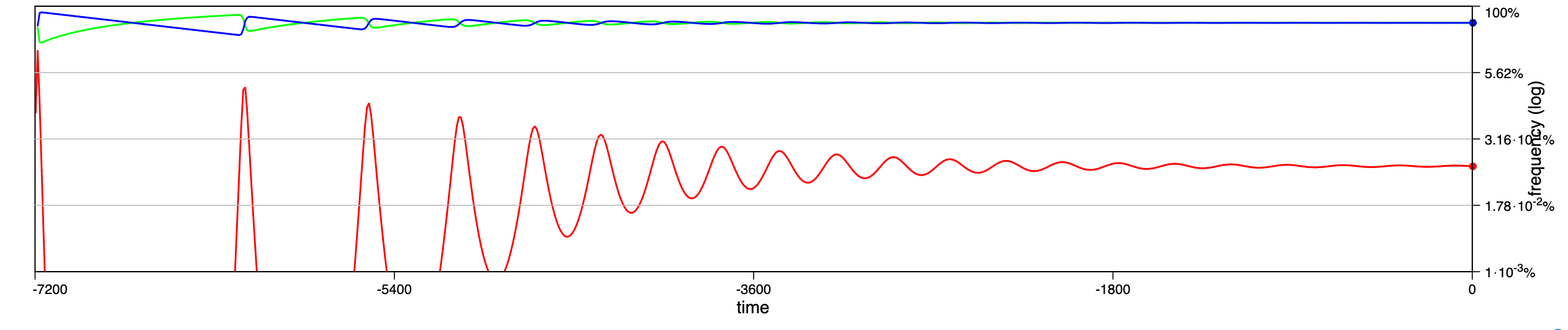
b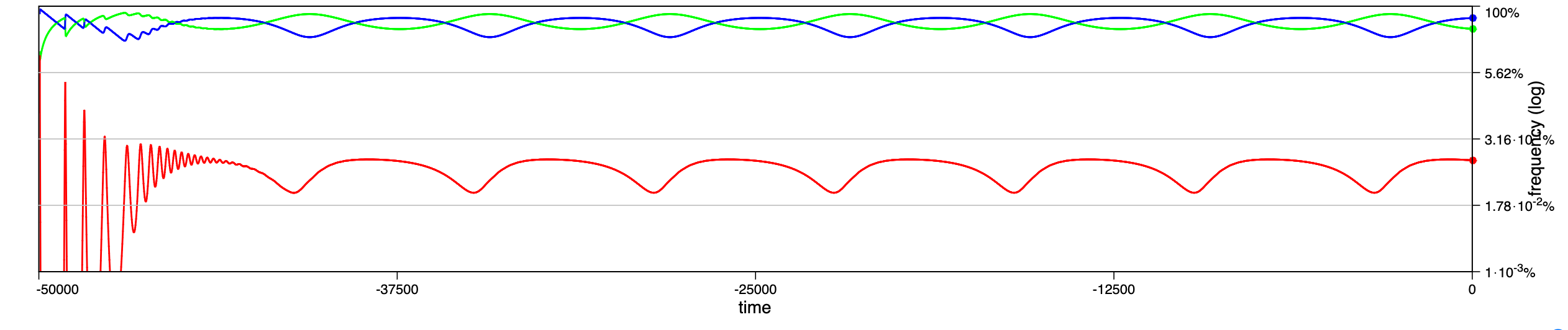
c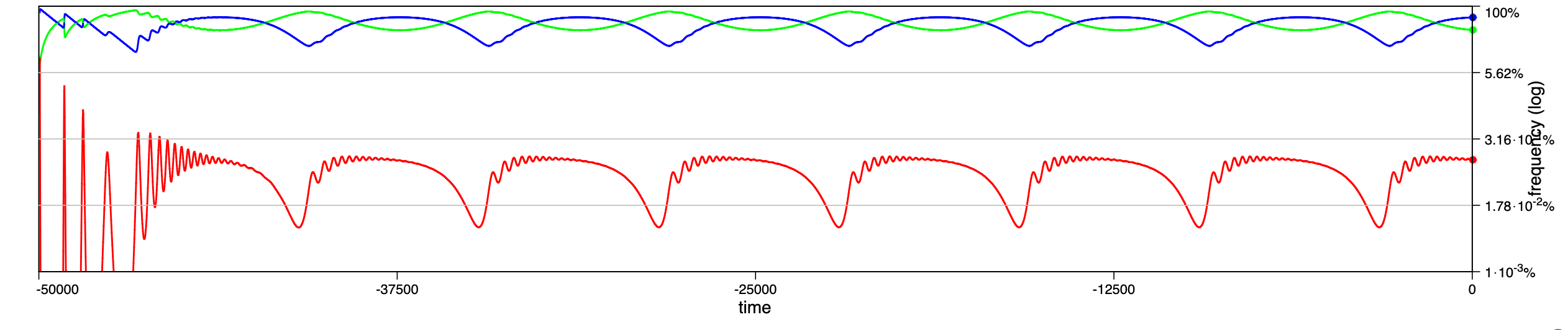
d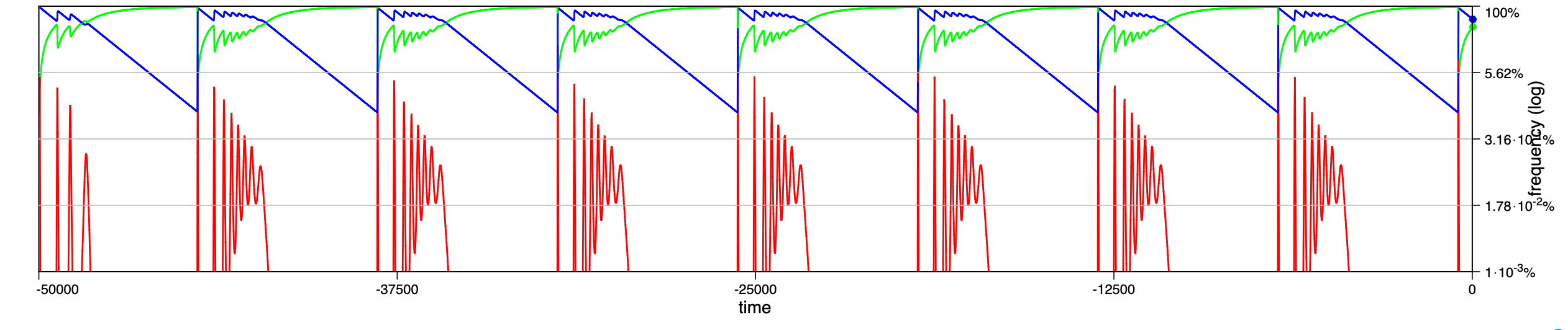
e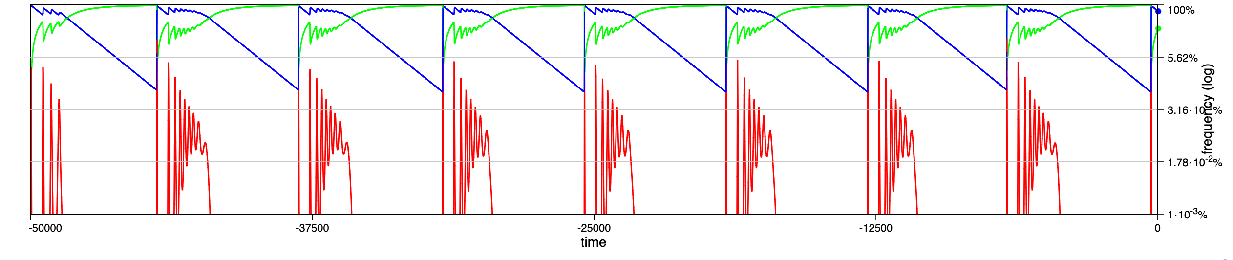
The results generated by the SIRE module are in fairly good agreement. The dynamics in panels a and b match perfectly; the damped, superimposed oscillations in panel c arise already at lower amplitude, ; while their irregular oscillations or spikes (compare panel d & e in Fig. 1 of Gai et al. (2024) with Fig. 14.2) are not observed.
-
Exercise 14.10:
Verify the reported results for and .
Hint Pay special attention to the --accurracy option, which controls the threshold for signalling convergence. . . Note: In principle, smaller values are preferred, but this increases the risk that the convergence criteria may never be met due to numerical rounding errors. . Solution Working parameter settings are ’--module SIR --model ODE --infect 1,<A>,0.001 --recover 0.5 --suscept 0.001 --init frequency 99,1,0 --accuracy 1e-5 --timestep 10’, where <A> is replaced by the desired amplitude. -
Exercise 14.11:
Assuming that you managed to verify and reproduce the results in Fig. 14.2, what are your observations?
Hint Use the context menu to change the -axis to a logarithmic scale.
The reasons for the discrepancies for larger amplitudes are most likely small differences in the implementations of the numerical integrator, combined with the fact that the density of infected individuals drops to extremely low levels, which makes the results sensitive to numerical inaccuracies.
14.9.5 Notes on small numbers and biological relevance
Let us conclude this section with a brief discussion of small numbers, numerical precision, and biological relevance. In the above exercise, the dynamics unfolds, rather reassuringly, largely as reported in Gai et al. (2024). However, the frequency of infectious individuals drops to less than for . This is an astronomical order of magnitude that even puts the Andromeda Strain to shame (Crichton, 1969). In an attempt to put this microscopic number into perspective, let’s return to the problem of exponential growth, see section 2.2: Population growth. We saw that a single E. coli bacterium would grow to a stunning cells over the course of merely two days – and weigh in at a few thousand times the mass of planet Earth. If merely one of these bacteria was infected, its frequency would amount to a massive fraction of as compared to . This just highlights that frequencies on that scale are utterly meaningless. In other words, it is always of crucial importance to put the results into perspective, and discuss them in the context of the biological scenario that inspired the model. While the mathematical findings remain valid and intriguing, their epidemiological relevance is questionable at best.
Moreover, small numbers are often a source of numerical instability. In java the smallest representable value with double precision is Double.MIN_VALUE, which is approximately . Problems easily arise when adding or subtracting numbers that differ by many orders of magnitude. For example, adding to will simply return because the difference is too small to be represented with double precision. As a consequence, the sequence when adding terms can matter such that for . This is called catastrophic cancellation and can lead to significant numerical errors.
The frequency of infected individuals in the above example is getting close to the smallest representable values, whereas the frequencies of susceptible and recovered individuals are of the order of . Given this huge difference, it is actually surprising that the numerical results remain stable.
14.10 Extension II: Oscillations and spatial patterns
Hopf bifurcations and Turing patterns are fascinating dynamical phenomena that arise when fixed points lose their stability: on the one hand, when a stable focus loses its stability, a Hopf bifurcation can give rise to limit cycles and oscillatory behaviour; on the other hand, Turing patterns emerge when a stable, homogeneous equilibrium becomes unstable due to diffusion-driven instabilities, which can give rise to the spontaneous formation of spatial patterns. Turing instabilities are relevant for all kinds of pattern formation in nature, ranging from patchy vegetation in arid areas (Rietkerk et al., 2004, Scanlon et al., 2007) to the spots of the leopard (Gell-Mann, 1994). Both phenomena are of great interest in various fields, including epidemiology, ecology, and evolution.
Neither Hopf bifurcations nor Turing patterns are observed in our basic model. Depending on the parameters, the dynamics either converges to an endemic equilibrium, – if it exists, it is globally stable – or the dynamics ends up in the disease-free equilibrium. However, it is relatively straightforward to modify the model to exhibit both Hopf bifurcations and Turing patterns by introducing non-linearities in the infection process. For example, by considering non-linear incidence rates, , which recovers our standard bi-linear setup for (Liu et al., 1986).
Because our population size is conserved, we have actually only two dynamical variables, say and , while can be eliminated through . Rewriting Eq. (14.2) accordingly, and including the non-linear incidence rates, we obtain:
| (14.4a) | ||||
| (14.4b) | ||||
Solving this dynamical system in general is a challenging task. However, at least for integer and we can still get some analytical traction, as we will see.
Note that the primary motivation to introduce these non-linearities was to better match empirical observations of disease outbreaks. They were first considered by Wilson and Worcester (1945b, a), who emphasized that they made this change “to investigate the consequences of various assumptions when the laws are not known.” This is important because it implies that the mechanistic processes that would give rise to such non-linearities are not well understood. As a consequence, what amounts to a small change to the ODE model can be very challenging to implement in individual based simulations. We have seen in section 2.8: From finite to infinite populations and section 5.5: From finite to infinite populations that the mass-action principle, or a Kramers-Moyal system size expansion, provide a deterministic way to derive an ODE from microscopic reaction equations. However, the reverse process, i.e. to derive microscopic rules from a given ODE, is not unique in general: different microscopic rules can give rise to the same macroscopic dynamics.
As an example, one possibility to achieve a non-linear incidence rate, based on a mechanistic description, is to assume that a susceptible individual needs to come into contact with multiple infected individuals simultaneously to contract the disease. For two infected individuals, the reaction kinetics can be written as a three-body interaction:
and results in an incidence rate of . Arguments along these lines can only justify integer exponents or , while their biological, or epidemiological, interpretation and justification still needs to be supplied. Here we simply circumvent this problem by focussing solely on differential equations, and stick to the bi-linear incidence rates for individual based simulations.
In the context of the model, Hopf bifurcations can describe periodic outbreaks of a disease even in the absence of seasonal forcing (c.f. section 14.9: Extension I: Adding seasonal variation), while Turing patterns can spontaneously give rise to stable, but spatially heterogeneous, distributions of susceptible, infected, and recovered individuals, in cases where the ODE model predicts a stable, endemic equilibrium, .
In order to implement non-linear incidence rates, we introduce a new array incidence, which holds the two additional parameters, the exponents and , and defaults of for each:
14.10.1 Differential equation models
The non-linear incidence rates can be implemented by modifying the beginning of the method getDerivatives(...). The first few lines now look like the following:
| . | . | Note: The method Math.pow(x,y) computes for arbitrary real but it is computationally a surprisingly expensive operation. Thus, the check ensures that it only gets called if a non-linear incidence rate has actually been set. | . |
14.10.2 Command line option
For convenience and to more easily explore the dynamics of the non-linear model, we add a command line option --incidence to set the exponents and . The parser accepts either one or two values, where the second value is optional and defaults to :
In order to advertise the new command line option, we also need to modify the method collectCLO(...) and append the following lines:
| . | . | Note: The option --incidence is only added if the selected model is not an individual based simulation, because non-linear incidence rates are much harder to implement and motivate in the mechanistic framework of IBS models. | . |
14.10.3 Hopf bifurcations & limit cycles
Now that we have the non-linear model in place, we can explore its dynamics. Some preliminary analytical considerations are helpful to guide our numerical explorations, and help focus on interesting parameter regimes. Let us begin by finding the equilibria and their stability in the ODE model, Eq. (14.4). However, let us also focus on a more manageable specific example with and all other transition rates positive, as well as and . The latter corresponds to the case mentioned earlier, where it takes two infected individuals to transmit the disease to a susceptible individual.
Due to the non-linearity, there may now be more than one interior equilibrium. In fact, for our specific example, there are three equilibria, one of which is the disease-free equilibrium, (assuming waning immunity, ), and two endemic equilibria, :
| (14.5) | ||||
The Jacobian matrix of Eq. (14.4) is
| (14.6) |
Interestingly, due to the non-linearity with , the disease-free equilibrium, , is now always stable (with eigenvalues and ).
At both endemic equilibria and holds. This simplifies the Jacobian to
| (14.7) |
The determinant of is then given by
| (14.8) |
and changes sign at
Conversely, using at with and , we obtain
| (14.9) |
Applying Vieta’s formula, the product of the two roots is given by
| (14.10) |
Thus, the determinant at the equilibrium with fewer infected individuals, with , is always negative and hence unstable, while it is positive at the other endemic equilibrium, with . The stability of the latter depends on the sign of the trace of . If is stable, , the system is bi-stable with two attractors, and . For a Hopf bifurcation occurs with
| (14.11) |
For larger , the trace is positive and unstable. In this case, the dynamics may converge to a stable limit cycle around , or renders globally stable again.
a

|
b

|
c

|
d

|
-
Exercise 14.12:
Consider the case with (recovery within days, on average) and (resistance lasting days, on average). For increasing infection rates, , show that
-
(a)
at low infection rates the disease-free equilibrium, , is a global attractor (e.g. for );
-
(b)
exhibits bi-stability between extinction and a stable limit cycles at slightly larger infection rates, (e.g. for );
-
(c)
bi-stability with a stable endemic equilibrium, , at large infection rate (e.g. for ).
For comparison, see Fig. 14.3.
-
(a)
14.10.4 Turing patterns
The ODE Eq. (14.4) can be easily extended to a reaction-diffusion system:
| (14.12a) | ||||
| (14.12b) | ||||
where and are now functions of a 2D spatial domain, denotes the diffusion operator, and the diffusion coefficients of susceptible and infected individuals, respectively.
Finding parameter combinations that promote the formation of Turing patterns requires careful considerations. In particular, the ODE model must exhibit a stable, endemic equilibrium. In our case the only candidate is , as we have seen in the previous section. More specifically, this requires that and at . Moreover, the diffusion coefficients of susceptible and infected individuals must be sufficiently different.
In the vicinity of the linearized dynamics of Eq. (14.12) is given by:
| (14.13) |
where denote the deviation from , refers to the Jacobian Eq. (14.7) at and represents the eigenvalue of a spatial perturbation. Any spatial perturbation in the square domain can be decomposed into spatial modes of the form
where denotes the linear size of the domain with spatial eigenvalues and integer . Interestingly, the spatial dynamics is not necessarily stable, even though it is stable against homogeneous perturbations (i.e., or ).
For some , Eq. (14.13) may take on the form of an activator-inhibitor system (Pearson, 1993, Turing, 1952). Any deviation from is then amplified by the fast diffusion of activators, while suppressed by the slow moving inhibitors. These antagonistic forces can give rise to the spontaneous formation of complex spatial patterns
In the spatial model, the susceptibles act as activators, because local increase in their density promotes further infections. Conversely, the infected individuals act as inhibitors, because they cannot get infected again. Turing instabilities require that activators diffuse fast, while inhibitors diffuse slowly. Epidemiologically this makes perfect sense because infected individuals are often too sick to move around much, while susceptibles are healthy and mobile.
If we neglect the condition that should be integers, the minimum ratio of the diffusion coefficients is given by
and must exceed .
a

|
b

|
Parameters: a b . a, b . The initial configuration is a 2D Gaussian density distribution with a maximum of infected individuals at the centre and no recovered individuals. Space is discretized as square lattice (von Neumann neighbourhood) with fixed boundaries. The snapshots are taken at .
-
Exercise 14.13:
Recreate the snapshots in Fig. 14.4 and enjoy the mesmerizing beauty of the slowly unfolding spatial patterns.
Solution For panel a the parameter settings are ’--module SIR --model PDE --infect 5 --recover 0.2 --suscept 0.06 --incidence 2,1 --pdeN 101x --geometry nf --pdeD 5,0.25 --pdeL 100 --init sombrero 9,1,0;1,0,0’ and for panel b ’--module SIR --model PDE --infect 12 --recover 0.1 --suscept 0.01 --incidence 2,1 --pdeN 101x --geometry nf --pdeD 5,0.25 --pdeL 100 --init sombrero 9,1,0;1,0,0’.
14.11 Outlook and extensions
An interesting extension would be to consider a scenario with mortality. Initially, the population is at an ecological equilibrium where births and deaths balance each other. Unleashing an epidemic with increased mortality affects the disease progression – especially in structured populations – and promises interesting results with increased realism. As a consequence, the quantity is no longer conserved, and adds a new dimension to the model. In individual based simulations this also implies that whenever an individual dies, it leaves a vacant site behind. Thus, a fourth, vacant type would be required.
References
- The andromeda strain. Alfred A. Knopf, New York, NY. doi: 10.1037/h0020871 see: §14.9.5, item 14.10.
- Recurrent and chaotic outbreaks in sir model. European Journal of Applied Mathematics, pp. 1–13. doi: 10.1017/S0956792523000360 see: §14.10.1, §14.10.1, §14.9.4, §14.9.4, §14.9.4, §14.9.5.
- The quark and the jaguar: adventures in the simple and the complex. W. H. Freeman & Co, New York, NY. see: §14.10.
- Influence of nonlinear incidence rates upon the behavior of sirs epidemiological models. Journal of Mathematical Biology 23, pp. 187–204. doi: 10.1007/bf00276956 see: §14.10.
- Complex patterns in a simple system. Science 261 (5118), pp. 189–192. doi: 10.1126/science.261.5118.189 see: §14.10.4, §14.10.4.
- Numerical recipes 3rd edition: the art of scientific computing. Cambridge University Press, New York. see: §14.3, §14.3, §14.4.
- Self-organized patchiness and catastrophic shifts in ecosystems. Science 305, pp. 1926–1929. doi: 10.1126/science.1101867 see: §14.10.
- Positive feedbacks promote power-law clustering of Kalahari vegetation. Nature 449, pp. 209–212. doi: 10.1038/nature06060 see: §14.10.
- The chemical basis of morphogenesis. Philosophical Transactions of the Royal Society B 237 (641), pp. 37–72. doi: 10.1098/rstb.1952.0012 see: §14.10.4, §14.10.4.
- The law of mass action in epidemiology: ii. Proceedings of the National Academy of Sciences USA 31, pp. 109–116. doi: 10.1073/pnas.31.4.109 see: §14.10.
- The law of mass action in epidemiology. Proceedings of the National Academy of Sciences 31, pp. 24–34. doi: 10.1073/pnas.31.1.24 see: §14.10.