Chapter 11 EvoLudo Reference
11.1 Graphical user interface
This section provides a detailed and comprehensive overview of the interactive capabilities of the EvoLudo simulation toolkit.
11.1.1 Basic interface
The basic elements of the graphical user interface are marked and enumerated in Fig. 11.1.
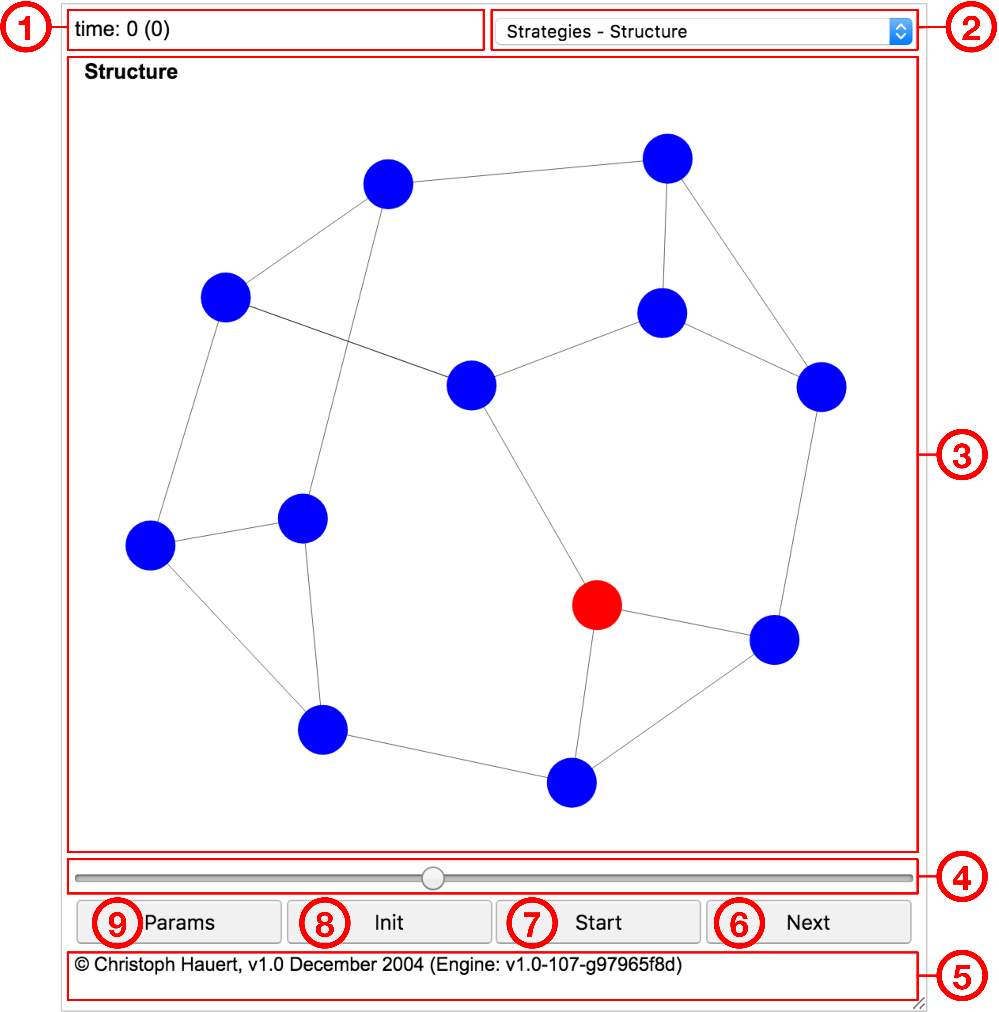
- ➀ Time:
-
Number of generations elapsed in individual based simulations. Each generation corresponds to updates, where denotes the population size (also known as a Monte-Carlo step). The continuous time equivalent is shown in brackets, where the fitness of the population determines the turnover rate and hence the timescale. For differential equation models a single number marks the elapsed time.
- ➁ View selector:
-
Numerous visualizations are available to explore the current state of the model, changes over time or statistical results. The selection of available visualizations depends on the details of the model.
- ➂ Visualization:
-
Graphical representation of various aspects of the model. For example, Fig. 11.1 shows the spatial arrangement of the Frucht graph ( nodes, each with three neighbours, for more information, see section 3.1.3: Graph symmetries and fixation times in the chapter on evolutionary graph theory) and two types of individuals coloured blue and red.
- ➃ Speed:
-
Adjusts the speed of running models. With the slider on the right the delay between subsequent updates is minimal ( msec) and maximal on the left ( sec).
- ➄ Settings:
-
Opens a panel with advanced controls to change the parameter settings of the model. For more information, see section 11.1.7: Advanced interface.
- ➅ Status:
-
Summary information about the state of the model. For many models this displays the current frequencies of each strategic type. The status line also shows alerts if warnings or errors arise when updating the model or when processing customized options.
- ➆ Next/Prev/Debug:
-
Advance the model by one single update. The size of an update step depends on the parameter settings and can be adjusted. Pressing the Alt-key (or with a long touch) the button changes to Debug for individual based simulations and takes a single microscopic update step and marks all individuals involved in the update. For models that permit time reversal, pressing the Alt-key (or with a long touch) the button changes to Prev and the model re-traces the previous step.
- ➇ Start/Stop:
-
Starts the model and periodically updates the graphical representation of the current state. While the model is running the button label changes to Stop for interrupting the model.
- ➈ Initialize/Reset:
-
Initializes the model. This sets the time to zero and restores the initial strategy distribution. When pressing the Alt-key (or with a long touch) the button changes to Reset, which also initializes the model but additionally regenerates the spatial structure. The latter only matters for randomly generated structures, such as random graphs (an example is shown in Fig. 11.2).
11.1.2 Views
EvoLudo offers various and versatile views to visualize (and manipulate) the current state of the model. The selection of available views depends on the active module. Two broad categories are modules based on a discrete set of traits (strategies) or on continuous traits. The following sections provide a detailed description of all available views.
Structures in 2D
![[Uncaptioned image]](figures/generated/gui-views-strat-struct.png)
Strategies – 2D Structure
![[Uncaptioned image]](figures/generated/gui-views-fit-struct.png)
Fitness – 2D Structure
Visualization of the population structure. Lattices have a fixed layout, while the layout of networks is dynamically generated. Typically, each node represents one individual and links define their neighbourhood. The node size scales with the number of neighbours: large nodes have many neighbours, while small ones have only a few.
In the Strategies – 2D Structure view the colour of each node indicates the strategy of the individual. For modules with discrete traits, each trait has a distinct colour and lighter shades mark individuals that changed their strategy during the most recent update. Colours can be customized with the --color option. For modules with continuous traits, the colour gradient represents the trait value.
In the Fitness – 2D Structure view the colour of each node indicates the fitness of the individual. The colour gradient ranges from low fitness () to intermediate () and high fitness (). Moreover, individuals achieving the same fitness as in a homogeneous population are coloured in a pale version of the corresponding strategy.
The layout is shared between the strategy and fitness views to simplify exploring and comparing the two visualizations.
The example shows a population of individuals arranged on a random graph with average degree and two types of individuals coloured blue and red. Note the light blue () and light red () nodes in the Strategies – 2D Structure view. The same colours are used to mark the fitness of those individuals in the Fitness – 2D Structure that perform equally well as in a homogeneous population of the blue and red strategies, respectively.
The views are interactive and respond to the following manipulations:
-
(i)
Hovering over a node with the mouse (tap on touch devices) displays more detailed information about the selected node. For example, in individual based models this includes the id’s of the node and its neighbours as well as the strategy of the individual, its fitness etc.
-
(ii)
Double-clicking on a node (double-tap on touch devices) changes the individual’s trait by cycling through all available strategies (only available in IBS models and modules with discrete strategy sets). This changes the current state of the simulation and is useful to introduce perturbations or generate particular initial configurations.
-
(iii)
Individual nodes in dynamically generated network layouts can be dragged (either with the mouse or one finger on touch devices) to adjust and fine-tune the network layout.
-
(iv)
The visible portion of a zoomed view is adjusted by dragging the view (tap and move). Note, in dynamically generated networks the initial click (or touch) needs to lie between nodes, otherwise the position of the node gets adjusted.
-
(v)
The mouse wheel (or pinching on touch devices) zooms in and out while maintaining the location of the mouse pointer (centre of pinching on touch devices).
-
(vi)
Right click with the mouse (two-finger touch and hold on touch devices) opens the context menu with further options to interact with the view, see section 11.1.4: Context menu. This includes the actions:
- Shake:
-
adjust the layout of dynamically generated networks by randomly moving nodes by a small amount and resume relaxation of the network,
- Full screen:
-
toggle full screen display of the GUI,
- Export…
-
export graphics or model configuration.
- Restore…
-
restore previously saved state of the model (property list, PLIST). This is also possible through drag’n’drop of the saved state onto the GUI.
For more information see section 11.1.6: Export & Restore.
Structures in 3D
![[Uncaptioned image]](figures/generated/gui-views-strat-struct-3d.png)
Strategies – 3D Structure
![[Uncaptioned image]](figures/generated/gui-views-strat-struct-3dana.png)
Strategies – 3D Structure (anaglyph)
![[Uncaptioned image]](figures/generated/gui-views-fit-struct-3d.png)
Fitness – 3D Structure
Visualization of the population structure in 3D. The colouring and sizes of nodes follow the same principles as in 2D representations of the population structure (see above).
The example on the right shows the exact same network as in the 2D view above. The 3D view offers equally rich interactive manipulations:
-
(i)
Hovering over a node with the mouse (tap on touch devices) displays more detailed information about that node.
-
(ii)
Clicking on a node (double-tap on touch devices) changes the individual’s strategy (not available for all models).
-
(iii)
The mouse wheel (or pinching on touch devices) zooms in and out, while preserving the location of the mouse pointer (centre of pinching on touch devices).
-
(iv)
Dragging the view with the mouse (one finger on touch devices) rotates the view in the corresponding direction.
-
(v)
Right click with the mouse (two-finger touch and hold on touch devices) opens the context menu with the same options as for the 2D view, see section 11.1.4: Context menu. However, 3D views offer some additional perks:
- Parallel projection:
-
toggle parallel (orthogonal) projection of population structure. The default is a perspective projection.
- Anaglyph 3D:
-
show structure as anaglyphs for an immersive 3D experience with your vintage red-cyan glasses. This works best if the view is in full screen.
- Virtual reality ():
-
split view into left eye and right eye views for 3D headsets. This experimental feature displays the network for each eye separately. In principle, it should work with a simple phone and Google cardboard. For more sophisticated 3D headsets possibly some tweaking might be required. However, no motion control is available at this time.
-
(vi)
The layout of networks and the current viewpoint is shared with the Fitness – 3D Structure view (see below) to simplify exploring and comparing the two visualizations.
Time series
![[Uncaptioned image]](figures/generated/gui-views-stratd-mean.png)
Strategies – Mean (discrete)
![[Uncaptioned image]](figures/generated/gui-views-stratc-mean.png)
Strategies – Mean (continuous)
![[Uncaptioned image]](figures/generated/gui-views-fitd-mean.png)
Fitness – Mean (discrete)
![[Uncaptioned image]](figures/generated/gui-views-fitc-mean.png)
Fitness – Mean (continuous)
Display the time series of traits and fitness. For modules with discrete traits the mean frequency and mean fitness of each strategic type is plotted over time. In addition, the fitness view includes the overall mean fitness of the population. For modules with continuous traits the mean trait value and the standard deviation are shown for each trait separately and the fitness view shows the overall mean fitness and the standard deviation of the population.
The discrete example shows the demise and extinction of cooperation in the donation game with cost-to-benefit ratio in a well-mixed population with individuals and initially defectors. Similarly, the continuous example shows the continuous donation game with linear cost and benefit functions with slopes and , respectively, and hence the same marginal cost-to-benefit ratio as the discrete example.
Interactive manipulations include:
-
(i)
Hovering with the mouse over the view (tap on touch devices) shows the coordinates of the selected point as well as information about the data collected at that time (if any).
-
(ii)
The mouse wheel (pinch on touch devices) zooms the horizontal axis in and out of while keeping the most recent time.
-
(iii)
The visible window of the horizontal axis can be shifted by dragging the view left or right (swiping with one finger on touch devices).
-
(iv)
The view is not cleared when clicking Init. This permits drawing multiple sequential trajectories. Use the context menu to clear the view or reset the model (Alt-Reset or touch and hold Init).
-
(v)
Right click with the mouse (two-finger touch and hold on touch devices) opens the context menu with further options to interact with the view, see section 11.1.4: Context menu. Most importantly this includes the action:
- Export…, Mean state (csv)
-
export the time series data to a CSV file.
For more information see section 11.1.6: Export & Restore.
Discrete strategies – 2D Phase plane
![[Uncaptioned image]](figures/generated/gui-views-strat-phase.png)
Strategies – 2D Phase plane
Depicts the dynamics of discrete strategy models in a 2D phase plane or phase plane projection. The two dimensions of the phase plane depend on the model.
The example shows a stable limit cycle in ecological public goods games (see section 7.5: Ecological Public Goods) in the phase plane spanned by the population density and the fraction of cooperators in the population.
-
(i)
Hovering with the mouse over the view (tap on touch devices) shows the coordinates of the selected point.
-
(ii)
For models that support it, a double click (double-tap on touch devices) initializes the model with the corresponding initial configuration. Note, with finite populations the state space is discrete and hence the exact location of the generated initial configuration may be a little off.
-
(iii)
Initializing the model does not clear the view. This allows to explore and illustrate the dynamics with multiple trajectories. Use the context menu to clear the view or reset the model (using Alt-Init or touch and hold Init).
-
(iv)
Right click with the mouse (two-finger touch and hold on touch devices) opens the context menu with further options to interact with the view, see section 11.1.4: Context menu. Most importantly this includes the actions:
- Time reversed:
-
reverse time if the current model permits (non-dissipative ODE and SDE models). This enables a more comprehensive exploration and visualization of the dynamics by tracing not only the future of a particular state but also its origins.
- Export…, Trajectory (csv)
-
export the data of the trajectory to a CSV file.
Discrete strategies – Simplex
![[Uncaptioned image]](figures/generated/gui-views-strat-s3.png)
Strategies – Simplex
The dynamics of models with three discrete strategies can be visualized on the simplex . Every point on the simplex indicates a particular composition of the population. The distance to each corner specifies the frequency of the corresponding strategy. Points closer to one corner indicate higher frequencies of that strategies. The corners represent homogeneous states of the population where all individuals adopt the same strategy. Edges represent population compositions with only two strategies. Each edge corresponds to a simplex spanned by the two strategies at its end points.
The example shows oscillations with declining amplitude in the Rock-Scissors-Paper game (see section 5.3.3: Rock-scissors-paper game).
-
(i)
Hovering with the mouse over the simplex (tap on touch devices) shows the frequencies of the three strategies at that point.
-
(ii)
A double click (double-tap on touch devices) initializes the model with the corresponding initial strategy frequencies. Note, with finite populations the state space is discrete and hence the exact location of the generated initial configuration may be a little off.
-
(iii)
Initializing the model does not clear the view. This allows to explore and illustrate the dynamics with multiple trajectories. Use the context menu to clear the view or reset the model (using Alt-Reset or touch and hold Init).
-
(iv)
Right click with the mouse (two-finger touch and hold on touch devices) opens the context menu with further options to interact with the view, see section 11.1.4: Context menu. Most importantly this includes the actions:
- Swap
-
swap the corners of strategies and .
- Time reversed:
-
reverse time if the current model permits (non-dissipative ODE and SDE models). This enables a more comprehensive exploration and visualization of the dynamics by tracing not only the future of a particular state but also its origins.
- Export…, Trajectory (csv)
-
export the data of the trajectory to a CSV file.
Fitness – Histogram
![[Uncaptioned image]](figures/generated/gui-views-fitd-histo.png)
Fitness – Histogram (discrete)
![[Uncaptioned image]](figures/generated/gui-views-fitc-histo.png)
Fitness – Histogram (continuous)
Display the current distribution of payoffs. For modules with discrete traits a histogram is shown for each trait separately. The bins that correspond to the payoff in a homogeneous population of the respective trait are marked by lightly coloured boundaries. The example on the right shows the payoff distribution for the donation game on a random graph with and average degree after five generations.
For modules with continuous traits a single histogram is shown with the bins marked that yield the minimum and maximum payoffs in a monomorphic population. The example on the right shows the payoff distribution for the continuous snowdrift game (see section 8.3: The continuous snowdrift game) in a well-mixed population after evolutionary branching gives rise to two distinct phenotypic traits.
Hovering with the mouse over the histogram (tap on touch devices) shows the boundaries of the selected bin as well as the proportion of individuals that fall into this fitness range.
Statistics
![[Uncaptioned image]](figures/generated/gui-views-stat-prob.png)
Statistics – Fixation probability
![[Uncaptioned image]](figures/generated/gui-views-stat-time.png)
Statistics – Fixation time
![[Uncaptioned image]](figures/generated/gui-views-stat-stat.png)
Statistics – Stationary distribution
The statistics views are only available for some models and require particular settings, such as well-defined initial configurations such that statistical samples can be collected. Selecting a statistics view will notify the model and potentially change the mode of execution. In statistics mode each step computes one statistics sample instead of a single update, see section 11.2.1: Modules, Models and Modes.
The first two examples show the fixation probabilities and times derived from samples for the spatial Moran process on a star graph with for a single mutant with fitness in a homogeneous resident population with fitness . The hub is the node with index and all leaves are indexed from to . If the initial mutant arises in the hub, it almost certainly disappears in the first updates. All other nodes are equivalent, and the variations are only due to stochasticity in the evolutionary trajectories of each sample. Note that the fixation probability is much larger than the expected fixation probability of approximately in a well-mixed population.
The third sample depicts a different kind of statistics. Fixation is only possible if absorbing states exist. Adding mutations eliminates the absorbing states but now permits stationary distributions. The distribution is shown for the same model as the fixation probability and time examples but with a small mutation rate of . Due to the long fixation times on the star graph even a small mutation rate is sufficient a significant fraction of population maintains the resident trait.
-
(i)
Hovering with the mouse over the histogram (tap on touch devices) shows the boundaries of the selected bin and more detailed information about the statistics.
-
(ii)
Right click with the mouse (two-finger touch and hold on touch devices) opens the context menu with further options to interact with the view, see section 11.1.4: Context menu. Most importantly this includes the action:
- Export…, Statistics (csv)
-
export the statistics data to a CSV file.
Continuous strategies – Histogram
![[Uncaptioned image]](figures/generated/gui-views-stratc-histo.png)
Strategies – Histogram
Displays the current distribution of continuous strategies in the population. The example shows a bi-modal distribution of investment levels in the continuous snowdrift game (see section 8.3: The continuous snowdrift game). Hovering with the mouse over the histogram (tap on touch devices) shows the boundaries of the selected bin as well as the frequency of strategies falling into that bin.
Continuous strategies – Distribution
![[Uncaptioned image]](figures/generated/gui-views-stratc-dist.png)
Strategies – Distribution
Displays the density distribution of continuous strategies in the population over time. The density is indicated by a colour gradient ranging from white for zero density to black, yellow and red for the maximum density.
The example illustrates the spontaneous diversification in the continuous snowdrift game (see section 8.3: The continuous snowdrift game). Evolutionary branching gives rise to the stable co-existence of high and low investing individuals.
Hovering with the mouse over the view (tap on touch devices) shows the range of the selected bin and the corresponding time. Only the most recent density is currently accessible for .
Structure – Degree
![[Uncaptioned image]](figures/generated/gui-views-degree-distr.png)
Structure – Degree
One of the most fundamental measures to describe the population structure (or the structure of any kind of network) is the degree distribution. The example shows the degree distribution of a random graph with average degree .
Console log
![[Uncaptioned image]](figures/generated/gui-views-console.png)
Console log
The console records all output of the model, including EvoLudo milestones (see section 12.10.1: Milestone listeners), warnings, errors, as well as debugging information. Most importantly problems when parsing command line options are displayed here to help resolve the issues. The verbosity can be controlled with the --verbose option, see section 11.2.2: Global options. Detailed help on all available command line options is also displayed in the console log when clicking Help or using --help.
11.1.3 Mouse manipulations and gestures
On touch devices, the EvoLudo interface recognizes the following gestures:
-
1.
Tap: Single short touch on the screen.
-
2.
Touch: Single extended touch on the screen.
-
3.
Two-finger touch: Two extended touches on the screen.
-
4.
Double tap: Two short touches on the screen.
-
5.
Drag: Touch and move on the screen.
-
6.
Pinch: Two-finger touch and move on the screen.
- Hovering, tap:
-
Display tooltip with more detailed information about location of pointer or tap.
- Double click, double tap:
-
Interact with view (if applicable). For example, to change initial configuration or alter individual traits.
- Right click, two-finger touch:
-
Open context menu.
- Dragging, touch and move:
-
Shift views (or nodes). Rotate structure in 3D views.
- Mouse wheel, pinch:
-
Zoom view.
11.1.4 Context menu
The context menu provides access to various options and functionalities depending on the active view. It is available by either clicking the right mouse button (or Ctrl-click) or a two finger touch gesture. Some entries may be inactive while a model is running. The following sections describe the available entries for each view type.
Common entries
The following entries are always part of the context menu:
- Full screen:
-
Enter full screen mode.
- Export…:
-
Export the data shown in the active view. Depending on the view, the following formats are available:
- State (PLIST):
-
Export the current state as an enhanced PLIST file. The saved state can be restored by drag’n’drop the exported PLIST file onto the EvoLudo GUI in a browser or by adding --restore <filename> to the command line options for a jar-archive.
- Vector graphics (SVG):
-
Export the graphics of the active view in SVG format.
- Bitmap graphics (PNG):
-
Export the graphics of the active view in PNG format.
- Trajectory (CSV):
-
Export the trajectory data of the active view in CSV format.
- Mean state (CSV):
-
Export the time series data of the active view in CSV format.
- Statistics (CSV):
-
Export the statistics data of the active view in CSV format.
- Restore…:
-
Opens a file viewer to select and restore a previously exported state of an EvoLudo simulation in the form of a PLIST file. Alternatively, the PLIST file can be dropped onto the EvoLudo GUI.
. . Note: Due to security restrictions imposed on JavaScript running in a web browser, it is not possible to specify and restore the state from a PLIST file using a command line option. For this reason, the option --restore is only available for java applications. .
Structure views
For views visualizing population structures, Strategies – 2D/3D Structure and Fitness – 2D/3D Structure, the following context menu entries are available:
- Shake:
-
shake network to assist with the relaxation of the layout process.
- Animate layout:
-
animated the layouting process.
- Zoom in ():
-
Enlarge the virtual view by a factor two. The virtual view can be shifted by dragging with the mouse or moving a finger.
- Zoom out ():
-
Reduce the virtual view by a factor of two. The virtual view cannot be smaller than the original size.
- Reset zoom:
-
Reset the zoom level to the original size.
For population structures with fixed layout, such as lattices, the Shake and Animate layout menu entries are disabled.
3D views
- Parallel projection:
-
toggle parallel (orthogonal) projection of population structure. The default is a perspective projection.
- Anaglyph 3D:
-
show structure as anaglyphs for an immersive 3D experience with red-cyan glasses.
- Virtual reality ():
-
split view into left eye and right eye views for 3D headsets. This experimental feature should work with a simple phone and Google cardboard or more sophisticated 3D headsets. However, no motion control is available at this time.
Time series views
Time series data is visualized by the views Strategies – Mean, Fitness – Mean, Strategies – Simplex and Strategies – 2D Phase Plane. The display can be customized using the following context menu entries:
- Clear:
-
empty the buffer and clear the view.
- Buffer size…
-
Set the buffer size for the view. The buffer size determines the number of previous states that are stored and displayed as trajectories. In order to optimize storage, new states are only stored if they result in a visible change on screen. If the buffer size is exceeded the oldest entries are discarded. The available buffer sizes are , (default), , and entries.
- Zoom in ():
-
Enlarge the virtual view by a factor two. The virtual view can be shifted by dragging with the mouse or moving a finger (views Strategies – Simplex and Strategies – 2D Phase Plane).
- Zoom out ():
-
Reduce the virtual view by a factor of two. The virtual view cannot be smaller than the original size (views Strategies – Simplex and Strategies – 2D Phase Plane).
- Zoom in x-axis ():
-
Reduce the visible data range by a factor of two. The smallest visible data window cannot be less than ten data points. The visible window can be shifted by dragging with the mouse or moving a finger (views Strategies – Mean and Fitness – Mean).
- Zoom out x-axis ():
-
Double the visible data range. The largest visible data window is given by the buffer size. The visible window can be shifted by dragging with the mouse or moving a finger (views Strategies – Mean and Fitness – Mean).
- Reset zoom:
-
Reset the zoom level to the original size.
In addition, all views also offer the option to export the visualized data in CSV format.
view
For the simplex view it is possible to customize which traits are shown and in what order:
- Swap :
-
Swap the strategies and in simplex graphs, where and refer to the strategies of the edge closest to where the context menu was activated.
- Set trait to …:
-
Change the trait of the corner closest to where the context menu was activated from strategy to any other strategy. Only available for modules with four or more traits.
Phase plane views
For phase plane views the options of the context menu heavily depend on the mapping of the current state to the phase plane. For fixed mappings no additional options may be available while other models may provide one or more of the following options:
- Autoscale axis:
-
For density based models the range of the - and -axes are automatically adjusted to accommodate all data points in the buffer.
- X-axis trait…:
-
Select the trait to display on the horizontal axis. Some models may allow selecting multiple traits and display their sum.
- Y-axis trait…:
-
Select the trait to display on the vertical axis. Some models may allow selecting multiple traits and display their sum.
Histogram views
For histogram views the sole customization through the context menu provides is:
- Autoscale y-axis:
-
automatically adjust the -axis range.
In addition, all histograms also offer the option to export the visualized data in CSV format.
Miscellaneous views
In addition, some models may provide further, specialized entries in the context menu:
- Time reversed:
-
reverse time. Only possible for non-dissipative ODE and SDE models.
- Symmetric diffusion:
-
request symmetric diffusion in PDE models. The request can only be honoured on lattice structures because otherwise the notion of symmetries is meaningless. Symmetrical diffusion is computationally expensive and hence disabled by default. In special situations numerical rounding errors may result in a breakdown of symmetry for settings that exhibit deterministic chaos, see section 1.2.2: Order & Chaos.
11.1.5 Keyboard shortcuts
- 0:
-
toggle settings panel.
- 1-9:
-
switch to view with the corresponding index in the view selector.
- Alt:
-
toggles mode of buttons.
- Esc:
-
does the first action in the following order: (i) exit full screen, (ii) stop running simulations, (iii) close settings panel, (iv) close popup EvoLudo view.
- Backspace, Delete:
-
stop running simulations, initialize (or reset if Alt is pressed) stopped simulations.
- Return, Space:
-
start or stop simulation.
- Shift Return:
-
applies new settings (if settings field has the focus).
- +, =:
-
increase speed, reduce delay between updates.
- -:
-
reduce speed, increase delay between updates.
- C:
-
export CSV data (if supported).
- D:
-
perform single, verbose debug step.
- E:
-
export current state of stopped simulation.
- F:
-
toggle full screen.
- H:
-
show help screen.
- n, →:
-
advance single step.
- P:
-
save PNG snapshot (if supported).
- p, ←:
-
backtrack single step (if model allows it).
- S:
-
save SVG snapshot (if supported).
- s:
-
shake network (if applicable).
11.1.6 Export & Restore
The current state of an EvoLudo simulation can be saved in an enhanced property list, PLIST-file, using the Export… ¿ State (PLIST) context menu of the graphical user interface, GUI, or the --export option of the command line interface, see section 11.1.4: Context menu and section 11.2.5: Simulation options. The PLIST-file is a simple, human-readable, and machine-parsable format which stores all settings as well as the current state of the model as key-value pairs.
| . | . | The enhanced PLIST format: The enhanced PLIST format stores double floating point numbers as the exact bit-string of a long integer in <real> entries, marked by a trailing character L. An important consequence is that it is possible to resume a simulation at the exact point when the state was saved. The conversion from double to the string stored with the <real> key uses: Long.toString(Double.doubleToLongBits(double)) + "L" and the reverse: Double.longBitsToDouble(Long.valueOf(string)) to convert <real> entries back to double after removing the trailing L. | . |
A saved state is restored by dragging and dropping the PLIST-file onto the EvoLudo GUI, by selecting Restore… in the context menu, or using the --restore option of the command line interface.
11.1.7 Advanced interface
The elements of the advanced user interface are marked and enumerated in Fig. 11.2. The visibility of the advanced user interface is toggled by the Settings button (see Fig. 11.1).
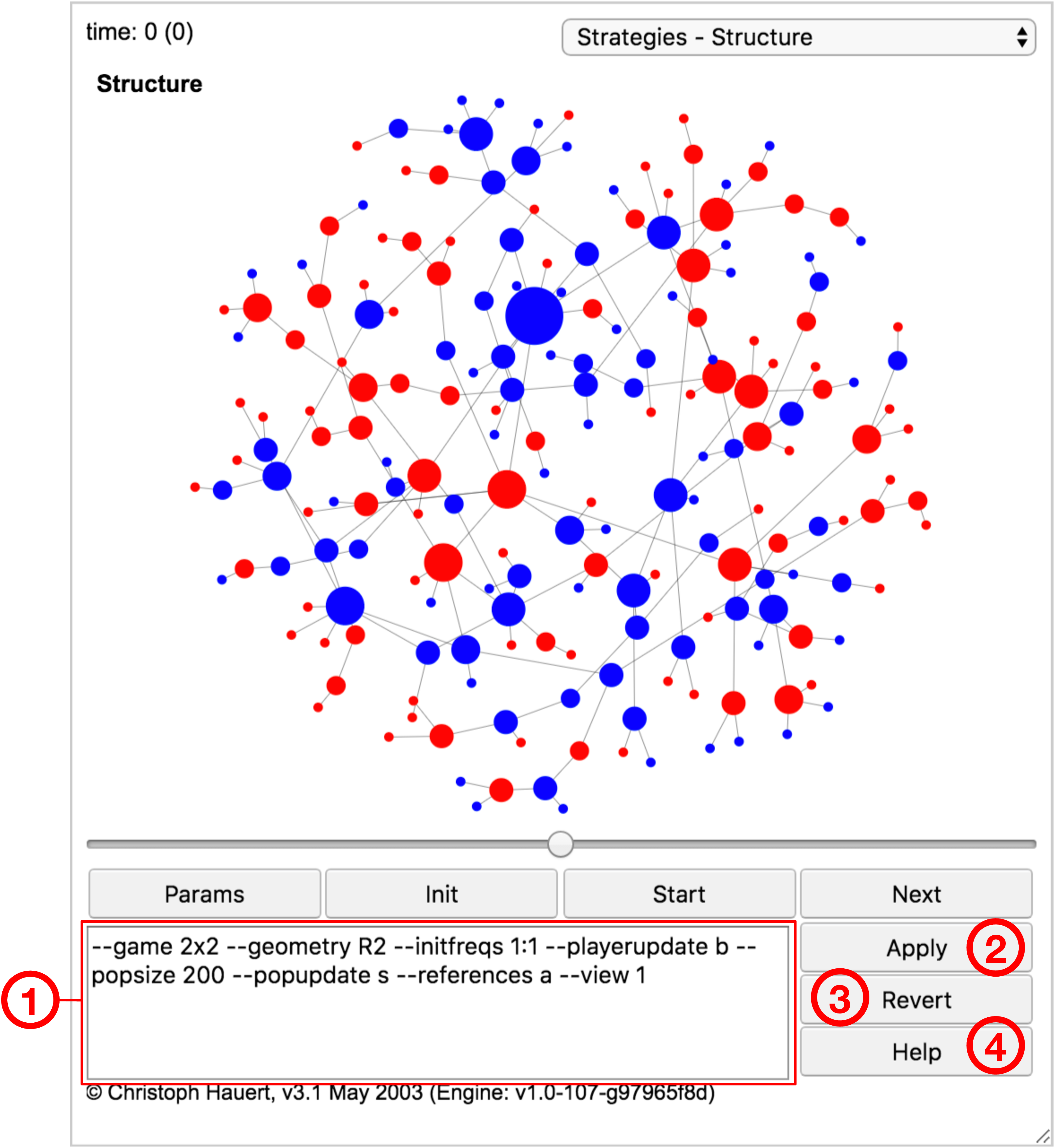
- ➀ Parameters:
-
Settings for the current model. These command line options are passed to the modelling framework and determine the type of model as well as aspects of its graphical representation (for a full list of options, see section LABEL:sect:XXX: LABEL:sect:XXX).
- ➁ Apply:
-
Applies the parameter settings to the model. Depending on which parameters have been changed, resetting the model may be required. For example, typically, when changing the geometry of the population a reset is necessary to generate the new structure, but when changing the payoffs of strategies the changes can be applied to the current state of the population.
- ➂ Default:
-
Discards any changes to the parameter settings and reverts to the default settings of this particular model.
- ➃ Help:
Note, for interactive labs embedded in the text flow of ePubs the parameters ➀ are read-only, the buttons ➂, ➃ are disabled, and the button ➁ displays Standalone, which opens a lab with identical parameter settings on a separate page where manipulations of parameters are possible (and the Console view is available, c.f. section 11.1.2: Views).
11.2 Parameters
11.2.1 Modules, Models and Modes
The EvoLudo toolkit has a modular structure, which allows the combination of different modules, models and modes. At the top are the modules, which refer to a particular evolutionary setup, for example, with constant selection, such as the Moran process, or frequency dependent interactions, such as games. Each model then indicates the kind of analysis of the evolutionary process. Depending on the module, this may include individual based simulations as well as numerical analyses based on ordinary, stochastic, or partial differential equations. Finally, the mode specifies the type of analysis: dynamics mode follows a particular evolutionary trajectory, while statistics modes collect samples from one or several realizations for statistical analyses. The availability of modes depends on further parameter settings, for example whether fixation can (or cannot) occur. Accordingly, the settings for the EvoLudo toolkit fall into the following categories:
- Global options
-
are available for all modules and models and determine general settings, section 11.2.2. This includes which module to load or setting the verbosity level of EvoLudo.
- Module options
-
specify the evolutionary game or process, section 11.2.3. This includes setting the interaction parameters, the payoff to fitness mapping, or selecting the model type.
- Model options
-
control the execution of the evolutionary process, section 11.2.4. This includes selecting the population geometry, the initial configuration, or the type of updates.
- Simulation options
-
determine the output of simulations, section 11.2.5. This includes setting the number of samples for statistics, the output location and precision, or restoring the state of a previous simulation.
- User interface options
-
are available to customize the graphical user interface, GUI, section 11.2.6. This includes setting names or colours for individual traits or selecting the initial view.
Each of the following sections describes the available options for the corresponding category. The options are listed in alphabetical order. The set of actually available options depends on the selected module and model.
11.2.2 Global options
- --help:
-
displays a summary of all available options.
- --module <module>:
-
loads the module <module> with all its settings. Available modules are
-
Moran
original Moran process with constant selection, see section 2.5.1.
-
2x2
games, see section LABEL:sect:XXX: LABEL:sect:XXX.
-
a2x2
Asymmetric games with environmental feedback, see section LABEL:sect:XXX: LABEL:sect:XXX.
-
RSP
Rock-scissors-paper games, see section LABEL:sect:XXX: LABEL:sect:XXX.
-
CDL
Voluntary participation in (non-linear) public goods games, see section LABEL:sect:XXX: LABEL:sect:XXX.
-
CDLP
Volunteering and punishment in public goods games, see section LABEL:sect:XXX: LABEL:sect:XXX.
-
CDLPQ
Peer and pool punishment in voluntary public goods games, see section LABEL:sect:XXX: LABEL:sect:XXX.
-
ePGG
Ecological public goods games with varying population densities, see section LABEL:sect:XXX: LABEL:sect:XXX.
-
CP
Centipede game for sequential cooperation and challenges to the notion of rationality through backwards induction.
-
Demes2x2
games in deme structured populations with migration between demes.
-
NG
Network games where the interactions between individuals encode the ephemeral population structure.
-
cSD
Continuous Snowdrift game, see section 8.3.
-
cLabour
Continuous Snowdrift game with two independent traits.
-
Moran
- --testRNG:
-
test random number generator.
- --verbose <l>:
-
set the level of verbosity for logging messages to the console. The level <l> is one of none, all, or in increasing order of severity debug/finest, finer, fine, config, info, warning, error. By default, messages at the info level or above are logged. The status line of the GUI displays the most recent message. More severe messages are never overwritten until EvoLudo is Reset.
11.2.3 Module options
The EvoLudo toolkit has a highly modular structure where every module represents a particular evolutionary setup. The following options are available for all modules. Module specific options are listed in section 11.2.7: Module specific options.
Common options
- --fitnessmap <m> [<b>[,<w>]]:
-
select the mapping of payoffs, , of individual to fitness, , with baseline fitness <b> and selection strength <w>. Available mappings are:
- --none:
-
no mapping
- --static:
-
static baseline fitness plus payoff contribution based on selection strength,
- --convex:
-
convex combination of baseline fitness and payoff contributions,
- --exponential:
-
exponential map,
The exponential mapping ensures positive fitness, regardless of the sign of payoffs. This is of the essence for transforming fitness into transition probabilities, such as in the original Moran process. Moreover, in the limit of weak selection it recovers the static mapping.
. . Note: --fitnessmap not available for modules with constant selection because no distinctions between payoffs and fitness are needed. .
- --model <model>:
-
activates the model type <model> and specific settings. Available models are
-
IBS
individual based simulations,
-
ODE
ordinary differential equations,
-
SDE
stochastic differential equations,
-
PDE
partial differential equations.
-
IBS
- --traitnames <n1[,n2...]>:
-
override the default trait names.
Discrete traits
- --disable <d1[,d2...]>:
-
disable traits with the specified indices. All traits are active by default.
Continuous traits
- --traitrange <min,max[;min,max]>:
-
restrict the range of traits to the interval [min,max]. By default, the range of all traits is set to .
11.2.4 Model options
EvoLudo offers different types of models that are selected using the --model option. Modules may not implement support for all model types. Each model comes with a set of options to control the execution.
Common options
- --seed[=s]:
-
set seed for random number generator. Setting the seed permits reproducible simulation results. If no argument provided the seed is set to . By default, no seed is set.
- --timerelax <r>:
-
set the relaxation time in number of generations, <r>. No relaxation by default.
- --timestep <s>:
-
set the report frequency to every <s> generations. By default, the report frequency is set to .
. . Note: For a report frequency of zero every single update in IBS models can be tracked. . - --timestop <h>:
-
halt execution after <h> generations. By default, execution continues indefinitely or until the model converges.
Individual based simulations, IBS: common
- --accuscores:
-
accumulate scores of multiple interactions. Payoffs are averaged by default.
- --addwire <a>:
-
add fraction <a> of graph links. No links are added by default.
- --consistency:
-
continuously check consistency of scores etc. This is computationally very expensive and should only be used for testing and debugging purposes.
- --geomcomp <>:
-
set the competition geometry (see --geometry). By default, the competition geometry is set to the same as the interaction geometry (see --geominter).
- --geometry <g>[f|F]:
-
set the population structure for interactions and competition. For lattices appending an (optional) f|F sets fixed boundary conditions (default is periodic). Available geometries <g> are:
- M:
-
mean-field/well-mixed population
- c:
-
complete graph
- l<l>[,<r>]:
-
linear lattice with <l> neighbours on either side if <r> omitted. Otherwise, asymmetric neighbourhood with <l> neighbours to the left and <r> neighbours to the right.
- n:
-
square lattice (von Neumann neighbourhood, )
- n2:
-
square lattice (second-nearest, diagonal neighbours, )
- m:
-
square lattice (Moore neighbourhood, )
- N<k>:
-
square lattice with <k> neighbours, where is , , etc.
- C<k>:
-
cubic lattice with <k> neighbours, where is , , etc.
- h:
-
honeycomb lattice
- t:
-
triangular lattice
- 0:
-
Frucht graph
- 1:
-
Tietze graph
- 2:
-
Franklin graph
- 3:
-
Heawood graph
- 4:
-
Icosahedron graph
- 5:
-
Dodecahedron graph
- 6:
-
Desargues graph
- s:
-
star (single hub)
- S<p[,a]>:
-
super-star with <p> petals and amplification <a>
- w:
-
wheel (cycle, single hub)
- +:
-
strong (undirected) amplifier
- -:
-
strong (undirected) suppressor
- r<k>:
-
random regular graph with degree <k>
- R<k>:
-
random graph with average degree <k>
- F<k[,p]>:
-
scale-free network (Klemm & Eguíluz) with average degree <k> and (optional) fraction of random links <p>
- f<k>:
-
scale-free network (Barabasi & Albert) with average degree <k>
. . Note: Sets the interaction and competition geometry to be the same structure. In order to set them individually use --geominter and --geomcomp. . - --geominter <>:
-
set the interaction geometry (see --geometry). By default, the interaction geometry is set to the same as the competition geometry (see --geomcomp).
- --migration <tm>:
-
set migration probability to <m> for migration type <t>:
-
none:
no migration
-
D:
diffusive migration (exchange of neighbours)
-
B:
birth-death migration (fit migrates, random death)
-
d:
death-birth migration (random death, fit migrates)
-
none:
- --optimize <t1[,t2,...]>:
-
enable optimizations:
-
none:
no optimization
-
homo:
skip homogeneous states (single species only)
-
moran:
update active links only (destroys timescale)
-
none:
- --playerupdate <u>:
-
select player update <u> (ignored by Moran updates, see --popupdate). The reference set is given by the --references option.
- best:
-
the focal individual adopts the trait of the best performing neighbour. If the fitness of the focal individual is better or equal to any of its neighbours the focal individual keeps its trait.
- best-random:
-
same as --best but ties are resolved by a coin toss.
- best-response:
-
the focal individual adopts the best-response strategy given the current reference set.
. . Note: Not available for continuous traits because of the computational complexity to determine the best response. . - imitate <s>:
-
the focal individual adopts one of the model traits/strategies with a probability proportional to the fitness difference. The selection strength <s> scales the fitness difference. For the maximum payoff difference results in adopting the model trait with certainty (or never in the opposite case). For the probabilities are truncated at and for the probabilities are confined to an interval around , which gets narrower decreasing .
- imitate-better <s>:
-
same as --imitate but only better performing model individuals are considered.
- proportional:
-
the focal individual adopts the trait of a model with a probability proportional to where the refers to the fitness of individual and the sum runs over all models, including the focal.
. . Note: The proportional update with exponential payoff-to-fitness mapping (baseline fitness of and selection strength ) is equivalent to the thermal <s> update with no mapping. . - thermal <s>:
-
the focal individual adopts one of the model traits/strategies with a probability based on the fitness difference, following the Fermi function:
where indicates the selection strength (inverse temperature), and are the fitness of the focal and the model individual, respectively. The probabilities are normalized to sum to one. The selection strength is controlled by <s>. For small selection is weak and reduces to a coin toss in the limit of . In contrast, for the probability of adopting the trait of a model with higher fitness approaches one.
. . Note: The imitate, imitate-better, and thermal updates all converge to the Heaviside step-function in the limit of strong selection large . . - --popupdate <u>:
-
select population update <u>
- synchronous <p>:
-
update fraction <p> of population synchronously;
- asynchronous:
-
update population asynchronously;
- once:
-
update every individual exactly once but in random order.
- Bd:
-
Moran process (birth-death, asynchronous).
- dB:
-
Moran process (death-birth, asynchronous).
- imitate:
-
Moran process (imitate, asynchronous).
- --popsize <n>|<nxn>:
-
set population size to <n> or <nxn>, which is convenient for lattices. The default population size is .
- --references <r>:
-
select the reference individuals that a focal individual uses to update its trait/strategy. Available reference sets <r> are:
- all:
-
all neighbours
- random <n>:
-
sample <n> random neighbours
- --resetscores <t>:
-
set the scheme <t> for resetting the scores to one of:
- onchange:
-
whenever an individual changes its trait;
- onupdate:
-
whenever an individual updates its trait regardless of whether this resulted in an actual trait change;
- ephemeral:
-
payoffs are determined and used only for updating.
- --rewire <r>:
-
rewire fraction <r> of graph links. No links are rewired by default.
Individual based simulations, IBS: discrete traits
- --init <t>:
-
set the initial configuration to type <t>, which corresponds to one of:
- frequency <f1,..,fd>:
-
random distribution of traits with frequency <fi>. If the module has more traits than the specified array has elements, the frequencies are applied in a cyclical manner and appropriately normalized. For example --initfreqs 2 sets equal initial frequencies, identical to uniform (see below).
- uniform:
-
distribute traits uniformly at random with equal frequencies.
- monomorphic <r>:
-
monomorphic initialization with resident trait <r>.
- mutant <m,r>:
-
monomorphic resident population with trait <r> and a single mutant with trait <m> placed uniformly at random. This corresponds to a mutational process where mutants arise spontaneously, for example due to cosmic rays.
- temperature <m,r>:
-
same as mutant <m,r> but mutant is placed on nodes with a probability proportional to their in-degree. This mimics a mutational process where mutants arise during reproduction and the mutant offspring is placed in a downstream node of the parent.
- stripes:
-
initialize the population with homogeneous stripes of all traits. This initialization guarantees boundaries between any combination of traits and is useful to explore the domain growth. Only available for planar graphs such as 2D lattices.
- kaleidoscope:
-
custom initialization available for select modules that produce evolutionary kaleidoscopes, see Lab. 1.1.
- --monostop:
-
stop simulations once population becomes monomorphic.
- --mutation <p> [temperature|random] [<t>]:
-
set mutation probability to <p> with temperature (during reproduction) or random (default) mutations. The available mutation types <t> are:
- none:
-
no mutations
- all:
-
mutate to any trait
- other:
-
mutate to any other trait
- range <r>:
-
mutate to adjacent traits, .
Individual based simulations, IBS: continuous traits
- --init <t>:
-
set the initial configuration to type <t>, which corresponds to one of:
- uniform:
-
uniform distribution of traits across the entire trait interval.
- mono <r>:
-
monomorphic initialization with resident trait <r>.
- gaussian <m,s>:
-
Gaussian trait distribution around mean <m> and standard deviation <s>.
- mutant <m,r>:
-
a single mutant with trait <m> in a homogeneous resident population with trait <r>.
- --mutation <p> [temperature|random (default)] [<t>]:
-
set the mutation probability <p>, the type of mutations (reproduction versus cosmic rays), and the mutational process <t> to one of:
- none:
-
no mutations.
- uniform:
-
uniform mutations to any trait value.
- gaussian <s>:
-
Gaussian mutations around parental trait with standard deviation <s>.
- range <r>:
-
uniform mutations around parental trait with range <r>.
Ordinary differential equations, ODE
- --accuracy <a>:
-
accuracy to determine convergence of trajectory . Numerical integration stops if .
- --adjusted:
-
adjusted replicator dynamics (instead of standard).
- --dt <t>:
-
set the step size of time increments to <t>.
- --timereversed:
-
integrate the dynamics backwards in time. This is useful for finding unstable fixed points in models that permit time reversal.
Stochastic differential equations, SDE
- --dt <t>:
-
set the step size of time increments for the integration to <t>.
- --timereversed:
-
integrate the dynamics backwards in time. This is useful for locating source areas in models that permit time reversal.
| . | . | Note: Trajectories in stochastic differential equations never converge to a fixed point, except for monomorphic absorbing states (in the absence of mutations), or extinction (for modules that include vacant space). | . |
Partial differential equations, PDE
- --accuracy <a>:
-
accuracy to determine convergence of the trajectory . Numerical integration stops if .
- --adjusted:
-
adjusted replicator dynamics (instead of standard).
- --dt <t>:
-
set the step size of time increments for the integration to <t>. Note, in PDE’s the step size may be decreased if it is incompatible with diffusion and/or advection terms.
- --geometry <g>[f|F]:
-
set population structure to <g>. The available geometries are the same as for individual based simulations, see above for a list and detailed descriptions. The default is a 2D square lattice with von Neumann neighbourhood, neighbours.
- --init <t>:
-
set the initial configuration type <t> to one of:
- uniform <f1,...,fn>:
-
set a uniform frequency/density distribution.
- perturbation <f1,...,fn>:
-
same as uniform but with a perturbation in the middle element with densities increased by a factor of or with frequencies inverted and normalized again.
- random <f1,...,fn>:
-
generate a random distribution, where each element contains frequencies/densities selected uniformly at random with <f1,...,fn> as the upper bound.
- square <f1,...,fn>:
-
place a homogeneous square with frequencies/densities <f1,...,fn> at the centre of an empty lattice for modules with vacancies and a lattice occupied by the dependent trait in modules without vacancies. The square has a side length of of the lattice side.
- circle <f1,...,fn>:
-
same as square but with a circular shape at the centre. The circle has a diameter of of the lattice side.
- sombrero <f1,...,fn>:
-
Gaussian density/frequency distribution with <f1,...,fn> at the maximum in the centre and embedded in vacant space or the dependent trait, respectively.
- ring <f1,...,fn>:
-
same as sombrero but with a donut-like distribution.
. . Note: All initialization types apart from uniform, random, and perturbation require a spatial metric and hence are only available for lattices. . - --pdeA <a00,...;a10,...,add>:
-
set the advection matrix for independent dynamical variables to , where aij indicates the advection of type towards for and away from for .
- --pdeD <d0,...,dn>:
-
set diffusion for independent dynamical variables to .
- --pdeL <L>:
-
set linear extension of spatial domain.
- --pdeN <N>:
-
set discretization of PDE ( bins for lattice side).
- --pdeSymmetric:
-
request symmetric diffusion.
. . Note: Requests for symmetric diffusion are only honoured by lattice geometries. .
11.2.5 Simulation options
For running simulations, EvoLudo provides a set of options to control the output and the execution of the simulation. However, most of these options are not available when running in a web browser. The reason is that due to security concerns the access of JavaScript code to the local file system is rigorously controlled and restricted. More information on running EvoLudo as a Java application can be found in section 12.2: Running simulations. Only options marked with * are also available in the web version of EvoLudo. The following options are available for controlling simulations:
- --append <filename>:
-
append output to file <filename> (default: stdout)
- --data <d[,d1,...]>:
-
type of data to report (default: none)
- traits:
-
traits of all individuals
- fithistogram:
-
histogram of fitness distributions
- traitmean:
-
mean traits of population(s)
- structdegree:
-
degree distribution of population structure
- scores:
-
scores of all individuals
- fitness:
-
fitness of all individuals
- statupdates:
-
statistics of updates till fixation
- fitmean:
-
mean fitness of population(s)
- stattimes:
-
statistics of fixation times
- statprob:
-
statistics of fixation probabilities
- --digits <d>:
-
set the precision of data output in number of decimal digits (default: 4)
- --gui:
-
launch legacy java application GUI (default: run in terminal)
- --export [<filename>]:
-
export final configuration of simulation to file <filename> (use %d to insert generation), (default: evoludo-%d.plist)
- --output <filename>:
-
redirect output to file (default: stdout)
- --restore <filename>:
-
restore saved state from file <filename>.
- * --samples <s>:
-
set the number of statistics samples to <s>. By default, the number of samples is unlimited.
- * --statistics <s>:
-
set statistics specific settings. The available setting types <s> are:
- reset <s>:
-
reset the geometry every <s> samples ( never). This setting is only relevant for population structures that involve random elements, such as random (regular) graphs. With reset 0 the geometry is never reset. By default, network geometries are regenerated for every sample.
11.2.6 User interface options
- --colors <c1;...;cd[;n1;...;nd]>:
-
array of colours to set the regular trait colours <c1;...;cd> for each of the traits and the colour when an individual newly adopts the trait <n1;...;nd>. If <n1;...;nd> is omitted and no new trait colours are specified, paler versions of the regular colours are used. Colours can be specified in different formats:
- grey:
-
the shade of grey is specified by a number .
- (r,g,b)-triplet:
-
the red, green and blue components of the colour are specified by numbers .
- (r,g,b,a)-quadruplet:
-
the red, green, blue and transparency (alpha) components of the colour are specified by numbers with opaque and fully transparent.
- named:
-
the available named colours are: blue, cyan, green, magenta, orange, pink, red, yellow, black, darkgray, gray, lightgray, white.
- --delay <d>:
-
set the delay between updates to <d> milliseconds. By default, the delay is set to milliseconds.
- --points <p>:
-
set the values of fixed points. Each point is specified as a -tuple for a module with traits. All fixed points are assumed to be stable unless any component is negative. Stable fixed points are shown as filled dots on phase planes or as dashed lines in time series as useful references. Similarly, unstable fixed points are displayed as open dots and dash-dotted lines, respectively. No fixed points are set by default.
- --run:
-
run simulations after loading of the module and model. By default, simulations are not started automatically.
- --size <w,h|fullscreen>:
-
set the size of the graphical user interface to width <w> and height <h>. By default, the size is set to pixels. Alternatively, the size can be set to fullscreen.
. . Note: The setting --size fullscreen requires user interaction due to security restrictions imposed on JavaScript and cannot be set programmatically. For this reason it works in the settings panel but not when e.g. included in a URL or a clo-data attribute that configures EvoLudo. . - --trajcolor <c>:
-
set colour for plotting trajectories, where <c> is the name of a colour, a grey scale value, , or a -tuplet with , see --colors above.
- --view <v>:
-
set the initial view to the view with index <v>. Instead of the index it is also possible to specify the name of the view with all spaces replaced by underscores, ‘_’. The available views depend on the module, the model, as well as the available modes. For a list of all EvoLudo views see section 11.1.2: Views.
11.2.7 Module specific options
Moran module
The classical Moran process with the trait indices of for the resident and for the mutant.
- --fitness <r,m>:
-
set fitness of residents to r and that of mutants to m in the original Moran process.
2x2 module
The classical games with trait indices of for strategy and for strategy .
- --paymatrix <a,b;c,d>:
-
set the payoff matrix to
The defaults are Axelrod’s classical payoffs for the prisoner’s dilemma with , and .
a2x2 module
Asymmetric games with environmental feedback. The payoffs of individuals not only depends on their strategies, or , but also on their environment, whether the individual is located on a rich, , or a poor, , patch. Effectively this results in four strategic types, , with indices . In addition, individuals may alter the quality of their patch by degrading good patches or restoring bad ones.
- --asymmetry <a>:
-
type of asymmetry
- g:
-
genetic (inherited) asymmetries
- e:
-
environmental (location dependent) asymmetries (default)
- --environment <g[,b]>:
-
location dependent payoff: g on rich and b on poor patches. The default is 0,0, no location dependent payoffs.
- --feedback <[,]>:
-
feedback between strategies and patches:
- :
-
restoration for strategy and
- :
-
degradation for strategy and
The default is 0,0,0,0, for no environmental feedback.
- --paymatrix <a,b;c,d>:
-
set the payoff matrix for interactions. Alternatively, specify a payoff matrix for strategies on rich and poor patches respectively: . The defaults are Axelrod’s payoffs 3,0,5,1.
Demes2x2 module
games in deme structured populations with migration between demes. The population geometry is restricted to the hierarchical type H, see section 11.2.4: Model options. The default is H1, which creates a single deme and hence corresponds to a well-mixed population.
- --migration <tp>:
-
set migration probability to p and the migration type t to one of:
-
B
birth-death migration, fit migrates, random dies
The default is B0.
-
B
- --paymatrix <a,b;c,d>:
-
set the payoff matrix (see module above).
RSP module
The classical Rock-Scissors-Paper game. The trait indices for the three strategies Rock, Paper, and Scissors, are
- --paymatrix <a11,a12,a13;a21,a22,a23;a31,a32,a33>:
-
set the payoff matrix to
The default is the standard Rock-Scissors-Paper game with
which results in closed orbits in the replicator dynamics.
CDL module
The public goods game with voluntary participation. Apart from cooperators and defectors this introduces a third strategy that abstains from social interactions and are hence termed loners. The indices of the three strategies are for loners, for defectors and for cooperators.
- --cost <c>:
-
the cost of cooperative contributions to the public good to <c>. The default cost is .
- --groupsize <n>:
-
set the size of interaction groups to <n>. The default group size is , that is, interactions in pairs.
- --interest <r[,rall]>:
-
set the multiplication factor of public good to <r>. When setting the optional second parameter <rall>, the multiplication factor is linearly scaled with the number of contributors. The default multiplication factor is .
- --lonecoop <c>:
-
set the payoff to a lone cooperator. The default payoff is to get the same payoff as a loner.
- --lonedefect <d>:
-
set the payoff to a lone defector. The default payoff is to get the same payoff as a loner.
- --loner <l>:
-
set the payoff to a loner. The default payoff is .
- --others:
-
no share of the benefit generated by an individuals’ contribution to the public good returns to the investor. By default, all participants get the same share of the benefit.
- --solo:
-
lone individuals also generate the public good (or not). This overrides --lonecoop and --lonedefect. By default, public goods interactions are social interactions and hence require at least two participants.
CDLP module
The public goods game with voluntary participation and peer punishment. In addition to the three strategies in module CDL this module includes peer punishers. Punishers contribute to the common pool but are willing to punish other individuals, but defectors in particular, at some cost to themselves. The trait indices are the same as in CDL plus the punishers with index . This module offers the same options as the CDL module above plus the following:
- --costpunish <c>:
-
set the cost of punishment to <c>. The default cost of punishment is .
- --leniencycoop <l>:
-
set the leniency towards punishing cooperators to <l>. The default is full leniency with . No leniency with a setting of .
- --leniencyloner <l>:
-
set the leniency for punishing loners to <l>. The default is full leniency with . No leniency with a setting of .
- --punishment <p>:
-
set the punishment/fine of defectors to <p>. The punishment of cooperators and loners is scaled according to --leniencycoop and --leniencyloner settings, respectively. The default punishment is .
CDLPQ module
The public goods game with voluntary participation and peer punishment. In addition to the four strategies in module CDLP this module includes pool punishers. Pool punishers also contribute to the common pool but in contrast to peer punishers they also contribute to a pool that is set aside to cover punishment expenses. The trait indices are the same as in CDLP plus the pool punishers with index . This module offers the same options as the CDLP module above plus the following:
- --costpoolpunish <c>:
-
set the cost of pool punishment to <c>. The default cost of pool punishment is .
- --poolpunish <p>:
-
set pool punishment/fine of defectors to <p>. The pool punishment of cooperators and loners is scaled according to --leniencycoop and --leniencyloner settings, respectively. The default pool punishment is .
ePGG module
Ecological public goods games with varying population densities.
- --cost <c>:
-
set the cost of cooperative contributions to the public good to <c>. The default cost is .
- --deathrate <d>:
-
set the rate at which individuals die in DE models to <p>. In IBS models this denotes the probability that the focal individual dies when picked to update. The default death rate is .
- --groupsize <n>:
-
set the maximum interaction group size for the public goods. The default group size is .
- --interest <r>:
-
set the multiplication factor of the public good to <r>. The default cost is .
- --lonecooperator <l>:
-
set the payoff to a lone cooperator to <l>. The default payoff to a single participant is .
- --lonedefector <l>:
-
set the payoff to a lone defector to <l>. The default payoff to a single participant is .
NG module
Network games where the interactions between individuals encode the ephemeral population structure.
- --ratio <r>:
-
set the cost-to-benefit ratio of cooperative actions in the donation game to <r>. The default cost is .
- --selection <s>:
-
set the selection strength for strategy imitation to <s>. The default cost is .
- --colors <a[;f[;e]]>:
-
set the colours for altruist (only provide help to others), egoists (only receive help), and fair players (same number of outgoing and incoming links) to <a>, <f>, and <e>, respectively. Each colour is specified by a colour name or an ’(r,g,b[,a])’ tuplet with r,g,b,a in 0-255. The default colours are green;yellow;red
CP module
The centipede game for sequential cooperation and challenges to the notion of rationality through backwards induction.
- --benefit <b>:
-
set the benefit of cooperation to <b>. The default benefit is .
- --cost <c>:
-
set the cost of cooperation to <c>. The default cost is .
- --nodes <n>:
-
set the number of decision nodes to <n>. The default number of nodes is .
SIR module
The classical epidemiological model with three compartments: susceptible, infected, and recovered. The trait indices are for susceptible, for infected, and for recovered individuals.
- --infect <i>:
-
the rate at with which a susceptible individual gets infected is set to <i>. This translates to a term for the increase in infected (and decrease in susceptible) individuals in differential equations models, where , and refer to the densities of susceptible, infected, and recovered individuals, respectively. For individual based simulations indicates the probability that a susceptible individual gets infected when encountering a single infected individual. When encountering multiple infected individuals, , the susceptible gets infected with the same probability, , in each encounter. More precisely, with probability the susceptible evades infection. The default is an infection rate of , which implies certain infection in individual based models.
- --recover <r[,s]>
-
the rate at which infected individuals from the disease and either become resistant, , or return to being susceptible, . This translates to terms and for the increase in recovered and susceptible (and decrease in infected) individuals, respectively, in differential equations models. Again, , and refer to the densities of susceptible, infected, and recovered individuals, respectively. The default is a recovery rate/probability of with everyone acquiring resistance in the process, .
- --resist <r>
-
the rate at which resistance wanes, and resistant individuals become susceptible again, . This translates to a term for the increase in susceptible (and decrease in resistant) individuals in differential equations models. As before, , and refer to the densities of susceptible, infected, and recovered individuals, respectively. The default is a recovery rate/probability of .
cSD module
The continuous snowdrift game.
- --benefits <t> <b0[,b1...]>:
-
set the benefit function type <t> for the focal individual’s trait and the opponent’s trait with parameters <b0[,b1...]>. The available benefit functions are:
-
0:
-
1:
-
2:
-
3:
-
4:
-
10:
-
11:
-
12:
-
13:
-
14:
-
20:
-
30:
-
31:
-
32:
-
0:
- --costs <t> <c0[,c1...]>:
-
set the cost function type <t> for the focal individual’s trait and the opponent’s trait with parameters <c0[,c1...]>. The available cost functions are:
-
0:
-
1:
-
2:
-
3:
-
4:
-
10:
-
11:
-
12:
-
13:
-
20:
-
0:
cLabour module
The continuous snowdrift game with two independent traits can result in spontaneous division of labour. The same cost and benefit functions are available as in the cSD module but now for two independent traits, , separated by a semicolon. For example --benefits 1 4.56,-1.6; 1 4.56,-1.6 and --costs 11 6,-1.4; 11 6,-1.4 to choose saturating, quadratic cost and benefit functions that are identical for both traits. Similarly, the initial configuration can be set independently for each trait. For example, use --gaussian 0.1,0.01;gaussian 0.9,0.01 to start with Gaussian distributions centred at and , respectively. If only a single function is specified it is applied to both traits.
The defaults are a linear benefit function for the sum of investments for both traits with , --benefits 10 3 and a linear cost function for both traits with , --costs 0 1. The default initial configuration is a uniform distribution over the entire trait interval for both traits, --init uniform.
11.2.8 Developers
- --consistency:
-
continuously check consistency of scores etc. This is computationally very expensive and should only be used for testing and debugging purposes.
- --mimic <f1[:f2[:...]]>:
-
emulate ePub modes and disable events:
- epub:
-
emulate ePub mode
- standalone:
-
emulate standalone ePub mode (for non-linear pages)
- nokeys:
-
disable key events (if available)
- nomouse:
-
disable mouse events (if available)
- notouch:
-
disable touch events (if available)
- --seed[=<s>]:
-
set the seed for the random number generator to <s>. This guarantees the same sequence of random numbers for repeatable simulations. Without the optional argument <s> the seed is set to . By default, no seed is set. More precisely, a random seed is set based on the current time.
- --snap [<s>[,<n>]]:
-
snapshot utility (uses capture-website tool). This adds ’<div id="snapshot-ready"></div>’ to <body> upon completion of the layouting process or after a maximum of <s> seconds or after <n> samples or generations, respectively.
- --testRNG:
-
perform several tests of the random number generator, see console for results.
- --verbose <l>:
-
set level of verbosity to <l> where the decreasing levels of verbosity are:
- all:
-
log all messages;
- debug/finest:
-
log messages at the finest level;
- finer:
-
log messages at the finer level;
- fine:
-
log messages at the fine level;
- config:
-
log configuration messages;
- info:
-
log information messages (as well as warnings and errors);
- warning:
-
log only warnings (and errors);
- error/severe:
-
log only errors;
- none:
-
turn logging of messages off.
The default is info.